Electronic properties

What can we learn from calculated MOs?

We have seen that we can display a LUMO
How reliable are calculated HOMOs and LUMOs?

In the HF approach, MOs are filled from the most stable upwards, until we get to the HOMO, when we have accommodated all the electrons
All the rest of the MOs are empty, 'virtual' MOs
The most stable empty MO is the LUMO

The number of occupied orbitals is fixed by the number of electrons, taken in pairs
If we use a bigger basis set, smaller percentages of more basis functions will be built in to this fixed number of occupied MOs
This should give a better description of each of these MOs, including the HOMO

Total no. of MOs = total no. of basis functions (i.e. contractions of gaussian primitives)
Therefore as we increase the size of the basis set, all the extra MOs are empty, virtual MOs

While the number of occupied MOs depends on the physical reality of how many electrons there are, the number of unoccupied MOs depends on the model, not on physical reality
The only requirement on the empty MOs is that they form an orthogonal set with the filled MOs
They are not optimised during the SCF process, because the energy of the molecule does not depend on them

Therefore, unoccupied MOs, including the LUMO, are much less reliable than occupied MOs, e.g. the HOMO

Natural bond orbitals

MOs are delocalised over the whole molecule
Usually they bear no resemblance to localised s and p bonds, or to lone pairs, so they cannot be used to support familiar chemical reasoning
Overlaps between hybrid orbitals to give localised bonds, invented by Pauling and used by practically all of the chemical world for human explanations ever since, are (fortunately) not just figments of our collective imagination: the calculated electron density can also be described in these terms
An ordinary MO calculation to get delocalised MOs is done at a high enough level to reproduce measured geometry or energies, then the atomic basis set is transformed into an equal number of natural atomic orbitals (NAOs), and the MOs into an equal number of natural bond orbitals (NBOs)
The additional transformations are cheap in computer time
This is called NBO analysis
It was devised by F. Weinhold, University of Wisconsin, during the 1980s
NBO is available in the Gaussian package
The process is:

AOs NAOs

Basis functions are transformed to natural atomic orbitals

NAOs NHOs

NAOs are combined into natural hybrid orbitals, so as to describe the atom's involvement in the calculated molecular electron density
The NHOs form orthogonal sets on each atom

NHOs NBOs

NHOs overlap to give NBOs

In this, the total number of orbitals stays the same:

ab initio

Because there is not a 1 to 1 correspondence between full or empty MOs and particular NBOs, the NBOs are not restricted to being either empty or full, as MOs are

NBOs have some fractional occupancy, between 0 and 2

Many NBOs contain nearly 2 electrons: these correspond to classical Lewis-type core or bonding or lone pair orbitals
Some of the remaining NBOs are not practically empty: usually these are antibonding orbitals

This corresponds to e.g.

NBO analysis can calculate the stabilisation energy coming from these delocalisations

This supports our ideas of donor p bonding, hyperconjugation, etc.

A (crude) contour plotting program, orbplot, is available on the UCS unix machines for visualising NHOs, NBOs, etc.
Although they are produced by objective mathematical transformations of ab initio MOs, NBOs look remarkably like the bonding, lone pair, or antibonding localised orbitals which we teach about
One use is to enable visualisation of non-bonded orbital interactions, e.g.

For an example of some NHOs, NBOs and stabilisation by delocalisation, see the separate web document NBO plots
If you have your unix id set up (see notes in Using Molden to view a geometry optimisation: it is assumed that you have done this exercise)

The instructions are given as the separate web document

Using more in unix to view an NBO analysis

Atomic charges

Atomic charge is not a measurable property of a molecule

Molecules do not consist of atoms, they consist of nuclei and electrons

Some arbitrary decisions have to be taken, on how to divide up calculated electron density between atoms
Consider a MO made of just two AOs, one on each of two atoms A and B

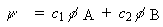
The electron density is the square of this:

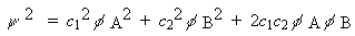
To find all the electron(s) in this, we integrate over the whole space of the molecule:

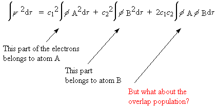
In Mulliken population analysis the overlap population is divided equally between the two partner atoms

This is arbitrary!
Often, bigger basis sets produce less believable Mulliken charges
Most electronic modelling programs calculate charges by the Mulliken method, because it is simple to do so

NBO analysis also calculates atomic charges, by summing occupancy of NAOs, but the results are different to Mulliken charges
A different approach is used to calculate ESP charges

Electrostatic potential, produced by the ab initio electron density, can be calculated at a grid of points
All the electron density can be treated equally in this: the only arbitrary decision is the size of the grid
Atomic charges, centred at the nuclei, which would produce the same set of potentials, are then found by least-squares fitting
ESP charges take longer to calculate, but do converge as basis set size is increased

Here are the atomic charges for methyl thiirane, calculated by these three methods:

Mulliken NBO ESP

C(H2) -0.521747     -0.55989     -0.342976
C(H)   -0.411345     -0.37339      0.038719
S       0.070747      0.11421     -0.192569
C(H3) -0.575628     -0.66843     -0.299563
H       0.222813      0.23979      0.117480
H       0.223591      0.23857      0.094816
H       0.212976      0.23279      0.097235
H       0.254341      0.25257      0.202466
H       0.257897      0.25664      0.170635
H       0.266353      0.26714      0.113758

Notice that only the method of fitting the electrostatic potential predicts a negative sulfur
How do we know which method to use?
We do not know. The best advice is to report only differences in charge distribution, between similar compounds

These are less likely to depend on method, and may be good enough to explain or predict trends