ACE1037 MACROECONOMIC SYSTEMS
[Cleaver, Chapters 2 and 3]
CONTENTS:
Comments,
questions and suggestions??
- The Market System & Circular Flow of Income: how do markets interact and generate economic flows?.
- Macroeconomics of the CFoI: The implications for government management of the economy - fiscal policy
- Money Market: Why money matters & monetary policy
- Interaction between Fiscal and Monetary Policy (IS/LM)
- Aggregate Supply/Aggregate Demand (a cautionary note)
- The Phillips Curve.
1.
The Market System
and the Circular Flow of Income.
The Market system works through specialisation
and trade:
People, communities, regions and countries are better off specialising
in production and trading the products with neighbours than they would
be if they tried to be completely self-sufficient. If this were
not
the case, markets would not exist.
Specialisation and Trade relies on people and their businesses
exploiting
their comparative advantage - specialising their productive
activities
in those areas and products for which they are best able, relative
to all the other things which they
might do instead. The comparison
implicit in comparative is with your own alternatives, not with the performance of
actual or potential competitors. Your own
opportunity
costs (what you could earn doing something else) should be less than
the returns you earn doing your
present
things.
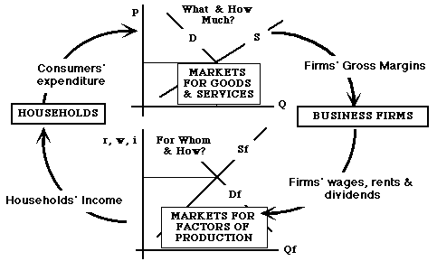
The general picture of interacting markets - the circular flow of
income:
- Households own the factors of production (land -
including
raw materials, labour, management and physical capital).
- Note - capital here means physical capital - plant,
equipment,
buildings
and machinery etc. (c.f. financial and money markets below)
- Households rent these factors to firms, in return for
income:
land rents; capital interest and dividend payments, and equity
appreciation
(capital gains); wages and salaries.
- Factor ownership provides income which fuels consumption and
demand in
the goods and services markets
- Firms rent the factors of production from households according to
their
demands for these factors, which is derived from the demands
for
the final goods and services
- Factor markets operate so as to encourage the owners of land,
labour,
manaement
and capital to rent out the services of the factors to the highest
bidder
- Firms add value to their own purchases of inputs and raw
materials.
They earn gross margins (total revenues minus cash input costs
[fuel,
power, packaging etc.] which is the value added to these inputs.
The Gross margin, or added value, or gross product
(each term means essentially the same thing for our purposes) is the
income
available to the fixed factors - land, labour, management and capital.
- In equilibrium, these returns will be normal profits - each firm
earning
sufficient to cover the opportunity costs of the factors of production
which they employ. If some firms or sectors are earning more than normal profits (those necessary to
persuade the participants to stay doing what they are already doing,
rather than doing something else), then more people and resources are
likely to come into this business, expanding supply, reducing prices
and profits.
[Note: profits in the everyday sense are, typically, just the
returns to capital - the earnings of the firms which are left after all
other legitimate costs (including labour and management costs) have
been
deducted. For self-employed family businesses, taxable profits
will
include the returns to the owners own labour and management, as well as
returns to the owners' land and capital, less allowable expenses in
servicing
mortgages, loans and debts. Economic profit is what is left after
further deducting the opportunity
costs of the owners' own capital, land, labour and management]
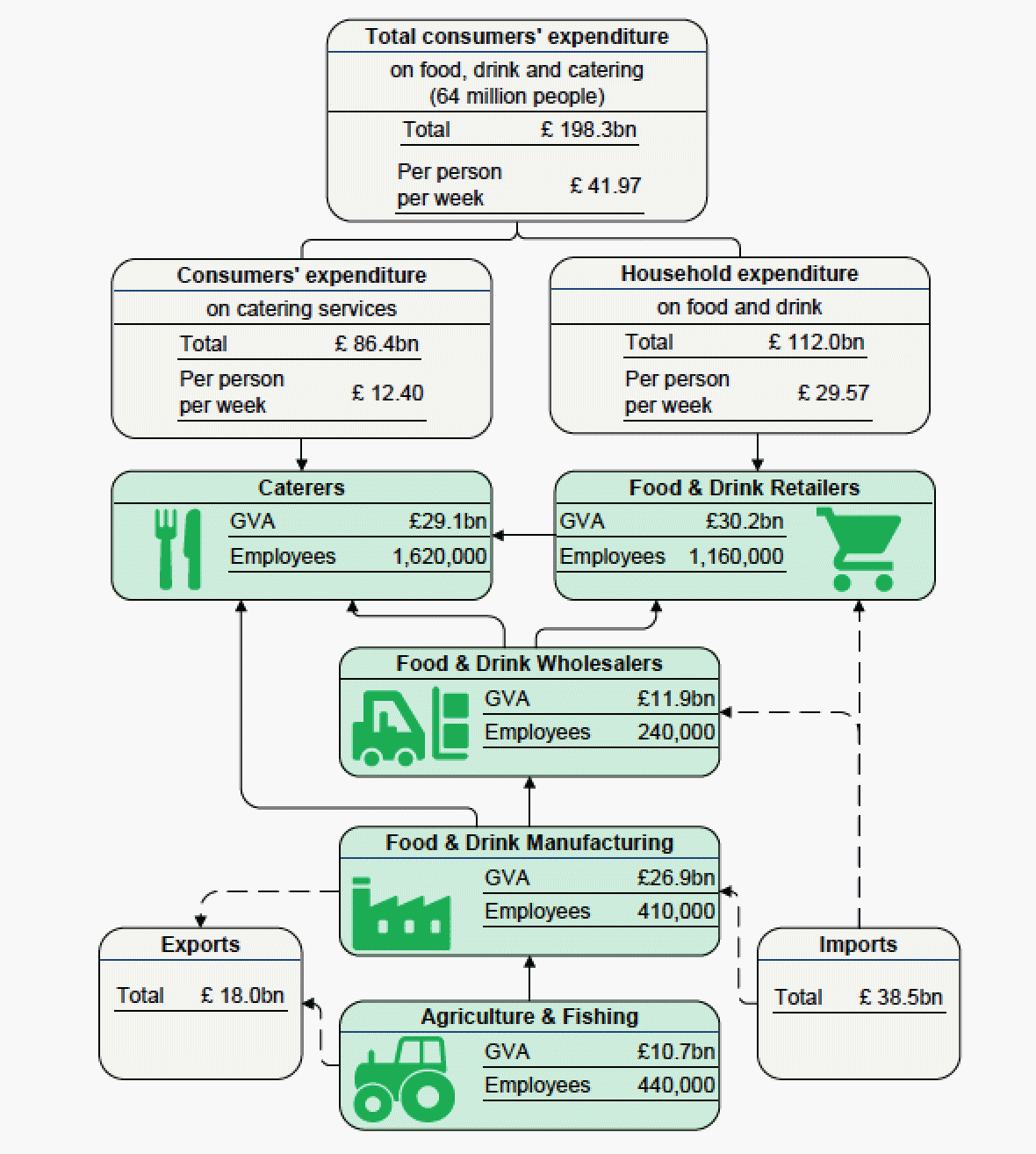
The UK food chain illustrates
the outcome of this circular flow of
income.
Agricultural and Food Chain, UK, 2016 (Defra, British Food and Farming at a Glance, April 2016).
 (Reconcilliation of these data with data for farming alone is slightly problematic)
From Defra's Agriculture in the UK, 2015, Table 4.1, (in real terms) p 20/21, UK farms produced:
£25.3bn total (gross) output (average over 2011-2015),
spent £16.1bn on purchased inputs (seeds, fertlisers, fuel, feed etc.)
leaving a gross margin ( Gross Product or Gross Value Added) of £9.2bn. (at market prices) on average. In comparison with the figure, this implies that the fishing industry produced a Gross Margin (GVA) of £1.5bn approx). In addition, the farm sector received £3.3bn as Direct Payments, environmental payments etc. on average over 2011-2015. Making a total of £12.5bn. as the GVA at factor cost.
This GVA (GM, Gross Product) represents the returns to the factors of production (land, labour,
management
and capital). Ag in the UK, Table 4.1 (ibid) identifies:
- Depreciation (Consumption of Fixed Capital) cost: £4.1bn.
- Interest (paid on loans): £0.36bn.
- Rent (as actually paid by tenants): £0.36bn.
- Labour payments: £2.5bn.
- Total £7.25bn.
- Leaving a 'surplus' of £5.2bn
as the "Total Income from Farming" (TIFF). This total income is
the reward (return) to farmers for their own labour, management,
capital investment and land ownership.
- Is it enough? Ag in the UK (ibid)
reports the total labour employed in the industry in Table 2.5
(p8). Depending on assumptions made about the proportions of
part-time, seasonal and casual labour which are equivalent to 1 full
time person, the implied annual wage for farm labour is somewhere
between £15k and £34k (divide the labour cost of £2.5bn. by the numbers
of regular labour, excluding farmers etc.) This same table also records
the number of farmers etc. trying to make a living from farming. Their
own labour is 'worth' between £4.3 & £6.8bn
at the implicit agricultural wage rate, leaving very little or nothing as a return
to land and capital. Similarly, Table 4.4 (p.27) reports on the
capital assets and liabilities of the industry. Total (average)
liabilities are £26.6bn. (in real terms) associated with an interest
cost of £0.36bn., an average interst rate of 2.47% (likely low because
of the predominance of long term liabilities). Applying this rate
of return to the reported total assets (capital investment) of
£242.6bn. generates a required return on own capital of £6.bn. [It
used to be possible to apply the same logic to land - applying the
average retns paid on rented land to the owned land area. However,
Defra no longer produce data on rented and owned land areas).
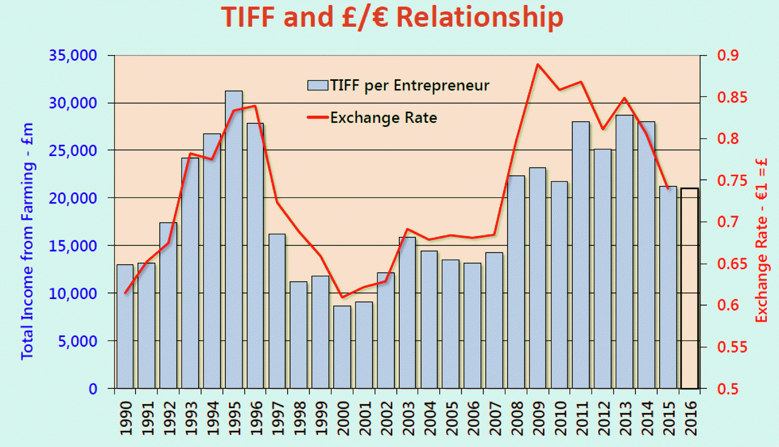
- TIFF varies quite substantially over time, and is
'currently' (2015) depressed by historical standards. The key
variable detemining TIFF in the short term is the £/€ exchange rate, as
pointed out graphically by Graham Redman of the Andersons Centre at the
2016 Agriculture in the UK Conference.
- In an exactly similar fashion, the input supply industries also process their own
inputs,
using
their own factors of production, producing their outputs (purchased by
the farm sector) and generating their own values added, as the incomes to their own land (including
natural
resources), labour, management and capital.
- Further processing by the Processing,
Distribution
and Retailing (PDR) sectors generates both values added (incomes to their own
factors)
and also the final output purchased by the final consumers.
- Thus, the final consumption figure (£198.3 bn.)
represents
the
cumulative total of all values added throughout the food chain,
and hence represents the total cumulative income earned by all
those
engaged in this food chain. (note
- the sum of the GVAs identified in the food chain figure above is well
short of the consumers' final spending, because the values added by the
input suppliers to each of the main sectors of the food chain are not
identified here.)
- Note that imports generate incomes in other countries rather than
the
UK,
while exports generate incomes in the UK.
Measurement Issues:
- Each of these flows (measured in £ bn.) represents a large
collection
of individual trades (prices times quantities): P
x Q
- Flows change through time because both prices and quantities
change: P1
x Q1 different from P2 x Q2
- Comparison between different years (periods) compares both price
and
quantity
changes
- Prices represent that rates at which quantities of one
good
or service
are exchanged for other goods and services - including the services of
factors of production (land, labour, management and capital), whose
prices
are rents, wages and salaries, and rates of return to capital.
- With prices set at some given, fixed level:
quantities
then
represent real income and real output of goods and
services
- the actual quantities of factor services which can be traded for the
purchase of actual quantities of goods and services - the purchasing
power
of each good or service in terms of all other goods and services.
- To measure these real quantities, prices (wages,
rents
etc.
as well as prices of goods and services) have to be fixed at some
given
level. - Pf. -> constant prices (volume) measures
- Comparison of Pf x Q1 with Pf x Q2 then shows the changes in
'quantities'
between Q1 and Q2.
- Also, comparison between Pf x Q1 and P1 x Q1 shows the difference
in
prices
between the fixed, constant, prices and those ruling in period 1.
- Notice - simply fixing the price of ONE good (say for
fertiliser),
allows
the actual physical quantities of fertiliser used by farms between
years
to be measured, but does NOT allow the measurement of the purchasing
power
of this fertiliser - to measure the purchasing power, we need
to
fix all prices at some constant level (typically using some
general price deflator - a price index measuring
changes in all prices - the Consumer Price Index, or the Retail Price
Index, or the GDP deflator. -> output and input flows in real terms. (See UK ONS Consumer price indices) & here for how the Consumer Price Index is calclulated.
Back to Contents.
2. Macroeconomic
Basics
- the Circular Flow of Income (CFoI) & Fiscal Policy
Simplify the whole economy as an interaction between Consumers
(households),
Producers (firms), and Government. NOTE: This is a
circular
flow of INCOME (and spending) - although measured and identified in
money
terms, it is the livings (income and spending) - the real
purchasing
power of the money - which is important here. Always refer to the
flow as an INCOME flow and not a flow of money.
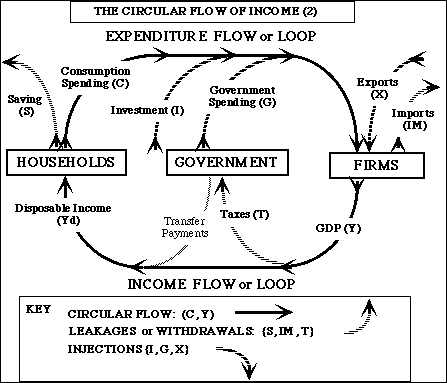
- Consumption (C) is spending on goods and
services for
final
use
(consumption) during this period.
- Investment (I) - an injection
into the
CFoI -
is the
purchase of actual physical capital (equipment etc.), or the
improvement
of peoples skills and expertise - final spending on things which are
intended
to increase income levels in future periods rather than this
one.
[Please Note: Firms are responsible for most of this investment,
not governments, though some government spending is investment for
future
periods rather than spending on current (this year's) goods and
services]
- Saving (S) is just and only income which is NOT
spent on
final goods
and services. (= Yd - C) - a withdrawal from the CFoI. [Please
Note: Investment spending is matched with Savings through the
financial
and money markets (see below), which are separate from this
Circular Flow of INCOME picture of the economy]
- Government Spending (G) is ONLY spending on final goods
and
services
(wages and salaries, paper, power, building maintenance and improvement
etc.) used up in this period or intended for use in future periods
(includes
any government investment) - an injection into the CFoI
- The other (major) part of total government expenditure is Transfer
Payments:
social security, unemployment benefit, public (national) pension
payments
etc. which simply add directly to the recipients incomes, and
which
are not paid in return for actual services.
- Taxes (T) are the government reciepts -
actually also raised
on
the
spending loop (VAT, excise duties), as well as on income streams
(income
and corporation taxes) - a withdrawal from the CFoI
- Exports (X) of goods and services provide
income for firms,
and
also
measure this part of total output of the economy - an injection
into the CFoI
- Imports (IM) of goods and
services leak income out of the
national (domestic)
flow of income - a withdrawal from the CFoI
- Total Expenditure equals
Output (C + I + G + X - IM) equals
Income
(called
Gross Domestic Product) (Y) which equals Disposable Income (Yd) plus
Taxes.
NOTE: Necessary Accounting equality (Total Expenditure =
Income)
over any one period (one year) does not necessarily imply equilibrium.
If Expenditure is growing, then so too will income - and both will be
larger
in the next period. If income is falling, then spending will also
fall, and both will be smaller next period.
Distinguish between
- trend growth (improvement in technology and productivity (outputs
per
unit
inputs)) typically about 2.5 - 3.5% per year
- cyclical growth (or decline) round the trend growth - booms
(strongly
positive
growth rates) and recessions (slower growth rates) or depressions
(negative
growth rates).
UK Real GDP (£m.) 1948 - 2015 (Source, ONS, UK National Accounts, Chapter 1 (Overview), Table 1.3)
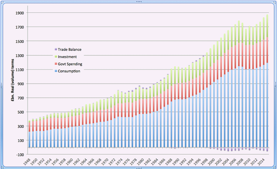
[Note: I have added Individual and Collective Government Final Expenditure to produce Govt. Spending here]
Note: 1973-74
depression (-2.5%, -1.5%) coinciding with entry to the EEC! - more
importantly, subsequent to the collapse of the fixed exchange rate
regime (1971), the 1st OPEC oil crisis and the major commodity price
boom. Followed, in 75-79, by a boom, and then another recession, and so
on. The 1994-2008 period of sustained growth still did not beat the
48-74 period (during fixed exchange rate period not withstanding
several devaluations).
You can find a wealth of macroeconomic statistics at the Treasury's Pocket Databank.
Equilibrium Process of the CFoI.
- Increasing Injections (G, I, X) and/or reductions
in Withdrawals (T, S, IM) will increase the CFoI
(increasing
income and output (expenditures) and vice versa. (hence the paradox of thrift - more savings meand lower incomes, unless these savings are invested in new plant, equipment etc.)
- Multiplier process - increasing an injection (for
instance)
increases
income, which then leads to further increases in spending and resulting
income
- until income levels have risen sufficiently that new
levels
of withdrawals
equal the new level of injections (increasing incomes tend to lead to
increased
savings, taxes and imports). Y (GDP) will not be in
equilibrium until
resulting Withdrawals balance Injections (see also, Economist, What is the Keynesian Multiplier (Sept. 2016)
Fiscal Policy as a stabiliser of economic cycles:
- Government Fiscal Policy (the balance between G and T) can
influence
equilibrium
Income levels
- Increase G (or reduce T) to counteract a recession
- Reduce G (or increase T) to counteract an unsustainable boom
(income
growth
exceeding full capacity of the economy, which leads to inflation - see
below)
Capacity Limits:
- Total Capacity of the economy to generate output and income
depends on
the quantities of land, labour, management and capital plant and
equipment
available
- When all of these factors of production are fully employed, the
economy
is operating at full capacity. Otherwise, there is unemployment -
the economy could produce more income and output.
- Capacity can be increased by:
- investment in capital plant and
equipment - more
capital for production and output;
- increase in the labour force
participating in
the economy - more employment -> more output & income;
- improvement in technology - more
output &
income from the same amounts of labour and capital through
technological
improvement - better quality and more productive capital;
- improved productivity of labour -
better skilled
and better organised labour increasing the amounts that can be produced
and the income that can be earned;
- structural change- re-organisation
of
resources
among different firms with lower costs, improving management.
- Fiscal Policy (G and T) can affect these
capacity increasing
processes - so should be used with care and caution.
Money and CFoI (and Inflation) - the simple story.
- Nominal National Income (GDP) [or GDP
Current terms] = P x Y
(a
grand sum of millions of price times quantity trades,
measured on the Expenditure loop). If all prices increase, then no-one
is any better off, in spite of the fact that nominal (current) GDP has
increased. Hence:
- Y
is real income - in terms of purchasing power over all goods
and
services, and P is the general price level (an index of all
prices
in the economy) (and is reported in national statistics as the GDP deflator - ask if you want to
know how this is calculated!)
- Money (M) is the medium through which
these trades
take place (notes, coins, and current accounts with banks).
- Money is a STOCK which is exchanged between
different
people and businesses as trades happen
- The FLOW of money round the CFoI is given by
M
x V, where V is the Velocity of Circulation - the number of
times
any one £ changes hands in the course of 1 year.
- MV = PY (the Quantity
equation of
exchange, or Fisher equation)
always holds - it is the only way of defining and measuring V.
- If V is constant (which is it,
approximately), then PY (nominal or
current
GDP, national
income) can only increase if M increases.
- If Y is fixed by the Capacity Constraint -
at Yf
(full
employment national income), then any increase in MV will lead to an
increase
in P - inflation.
Note: the Economist (Oct. 27, 2012) comments on the multiplier process
in the context of current austerity (shrinking budget deficits), which
you should be able to understand, at least in principle, from these
notes. A leader in the same issue also comments on the debates between
right and left (largely) about the sense of austerity in times of recession.
Note 2: This brief outline also serves to explain the GDP Deflator: (see, also, economics.about.com): The ONS statisticians can calculate National GDP at current (nominal) prices, and also at constant (real) prices, the latter using specific price indices for different categories of spending and income which go to make up the national GDP. At nominal prices, GDP = PxY, but using constant prices GDP = Y, with prices (P)
held constant at the base year. This re-calculation of GDP at constant
prices allows us to compare the nominal to the real value (PY/Y) for any given year, which gives us a measure (index) of the general average change in prices (P) between different years. - this is the GDP deflator.
Back to Contents.
3. Money Market
The Market for Money (Money market)
Money is used both as a medium of exchange for transactions (active
bank
balances) and also as a store of wealth & for precautionary purposes (idle bank balances).
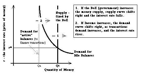
Demand
for and Supply of Money: The price of money is "the
interest
rate" (what we have to pay to get more of it!) in
quotes, because 'the interest rate' is actually a proxy for a wide
constellation of interest rates, depending on the risks and
credit-worthyness of the borrower, and the judgements and resources
(including the willingness of the central banks and governments to back
up and underwrite 'bad' loans) of the lenders.
- Demand for money (current account bank balances and credit limits) depends on:
- Income (especially for transactions or active balances)
- Price (the interest rate) especially for idle balances - the
higher the
interest rate, the greater the opportunity cost of holding wealth as
money
rather than as financial or physical assets.
- Money Supply is controlled by the Monetary Authority - the Bank
of
England
(BoE).
- Monetary Policy is decided by the Monetary Policy Committee of the
BoE,
with the objectve of controlling inflation
- either through controlling the Supply of Money directly (which
proves
to
be rather difficult)
- or by setting the base lending (interest) rate of the Bank of
England
to
the commercial banking system - the current system of Monetary policy.
(Setting the interest rate at a new level above r* will automatically
result
in a contraction of the supply of money to match the reduced demand -
since
the BoE, through its function as lender of last resort, implicitly sets
the
supply of money to match its ruling interest rate)
4. Interactions between Fiscal and Monetary Policy (IS/LM analysis)
Capital markets are the interaction between saving and
investment, given the rate of interest set by the Money Market
and Monetary Policy, other things being equal. Higher interest rates -> less investment & greater savings, and vice versa.
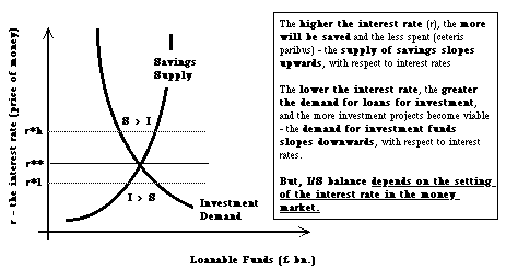
Interest Rates and the Circular flow of income - the
I-S Curve
But other things can never be equal in a flow system - the circular
flow of income. Because, when savings and investment change in the circular
flow, then income also changes. And income determines savings and
also influences investment - the more income an economy generates, the
greater the incentives to invest in new plant and equipment to provide
for new goods and services to satisfy the increased income.
So what? Suppose that Monetary Policy has set the interest rate "too
high" for an equilibrium between savings and investment - the rate is such
that there is a surplus of savings supply over investment demand. What
will then happen? Think about the circular flow of income - with leakages
or withdrawals from this flow (savings) greater than the injections (investment).
Income levels will fall in this case, and will go on falling until savings
comes back into balance with investment. How does this happen? As
income falls, so savings will fall as well, there being less income to
save. Eventually, income levels will adjust so as to bring the circular
flow back into equilibrium - so that savings do equal investment at this
"too high" interest rate. The consequence of the high interest rate is
to reduce income (Y), thus shifting the Savings curve in the Capital
Market, and probably shifting the Investment curve, too.
As Income changes, so the Savings supply and Investment demand curves
shift
in the capital market
The same argument works in reverse - a condition in which money market
interest rates encourage more investment than saving. In this case, income
levels in the circular flow will tend to increase, providing more savings
to match the level of investment encouraged by the interest rate.
In other words, income adjusts in the circular flow of income
to as to balance savings with the investment levels set by the interest
rate (which is determined in the money market). This is the essence of
the interaction between interest rates and the circular flow of income,
and can be represented by the
Investment-Savings (I-S) curve relating interest rates to
the level of national income (Y):
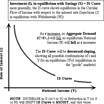 The IS curve shows
the equilibrium relationships between the rate of interest (established
in the money market) with the level of national income,
assuming
that
the remaining injections and withdrawals (G, T, X and IM) stay as before.
If these other (exogenous) injections and withdrawals
change,
then the IS curve itself will shift.
Thus, if government spending (G) is increased (and/or taxes (T) are
reduced) - an expansionary Fiscal Policy - and the IS curve will shift
to the right - because an expansionary fiscal policy will increase levels
of national income for each and all levels of savings and investment, each
and all levels of the interest rate.
The IS Curve slopes
downwards because lower
 interest
rates (r down) encourages investment and consumption and thus increases
 national
income (Y). It thus represents the combinations of r and Y which are consistent
with equilibrium in the goods and services markets (the circular flow
of income). Note this. The CFoI is, in effect, a description
of equilibrium in the markets for goods and services (and factors of production)
-equilibrium in the 'real' (non money) part of the economy.
Note, too: this curve is universally known as the IS curve -
but it should really be called the JW curve - the equilibrium
combinations
of interest rates and incomes in the CFoI, recognising that interest
rates
might also affect G, T, X and IM, as well as S and I. Interest
rates can have effects on Government spending and Taxes, and on IMports
and Xports, as well as on Savings and Investment in the domestic
economy.
A significant part of Government spending is on servicing the national
(Government) debt. Interest payments on government debt will
obviously change as the current interest rate changes. This can
trigger changes in tax to allow for the change in G.
UK interest rates versus interest rates elsewhere in the world can also
affect the Imports and Exports of, especially, services such as
insurance, commodity broking, financial and foreign exchange services
and so forth.
Money Markets and income changes - the L-M curve: As incomes increase, so the demand for money will also increase - more
income means more spending, which requires more money (or an increase in
the velocity of circulation - the efficiency with which the money stock
is used).
An increase in income will shift the demand curve for money to
the right (see above).
If the supply
of money is kept constant, and assuming that the velocity of money also
remains constant, then this shift to the right will increase the
interest rate. The same argument works in reverse - a fall in income
will reduce the demand for money, which will reduce interst rates, so long
as the money supply is held constant.
This relationship between income and the interest rate through
the money market is represented as the L-M curve - the Liquidity
preference (demand for money) and Money supply relationship:
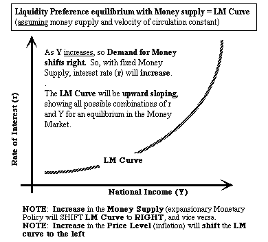 The LM curve shows
all those combinations of Y and r which are consistent with an equilibrium
in the Money Market (given a fixed money supply and a constant velocity
of circulation)
The LM curve will shift to the right if the money supply is
increased, or if interest rates are reduced, in the money market through
monetary
policy. An expansionary monetary policy shifts the LM curve to the
right. A contractionary monetary policy shifts the LM curve to the left.
Notice, too, the effect of inflation (an increase in the price
level (P)) on this relationship. If the price level increases in
the economy, then the stock of money in the economy cannot finance the
same level of real transactions as before. We will need more money
for any given level of Y at higher price levels than at low price levels.
With a fixed supply of money, the greater demand for money at a higher
price level means a higher rate of interest at a higher price level for
any given Y. So inflation shifts the LM curve to the left.
This is important - if you have not grasped the reasoning - try it again,
slowly.
IS and LM interactions
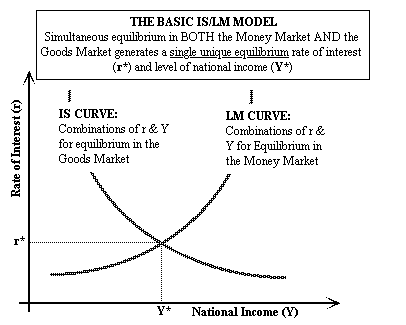
The IS curve captures the essential relationship between the rate of interest
and income in the markets for goods and services (the circular flow of
income). The LM curve captures the essential relationship between the rate
of interest and income in the money market.
For the two markets to be consistent with each other - the same rate
of interest ruling in both the goods and services market and in the money
market - there can only be one equilibrium level of national income
(Y*), shown by the intersection of the IS curve with the LM curve.
Links between Monetary and Fiscal
Policy
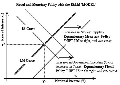
We now have the effects of:
-
Fiscal Policy captured in the IS curve (where an expansionary
fiscal
policy shifts the IS curve to the right, and vice
versa);
-
Monetary Policy captured in the LM curve (where an expansionary
Monetary
policy shifts the LM curve to the right, and vice
versa)
To see the effects of changing monetary and fiscal
policies, you should now experiment with this diagram. You will not understand
it unless you do it for yourself. Do it now.
You should get the following results. (If you do not, then try
again!):
-
Expansionary Fiscal Policy - shifts IS right: will tend to increase
Y and also increase the interest rate (r)
-
Notice that, because monetary policy (the money supply) is held constant
in this experiment, an expansionary fiscal policy forces the government
to borrow the difference between G and T from the private sector, and this
increased borrowing (or reduced lending to the private sector if T is greater
than G) means that the interest rate must increase.
-
Thus, given a constant monetary policy, the interaction between fiscal
and monetary policy will reduce the effect of the multiplier through
the effects of the interest rate on income levels - increased government
spending
crowds out private spending to some extent.
-
Contractionary Fiscal Policy - shifts IS left: will tend
to reduce both Y and r
-
Notice that the contraction in fiscal policy frees up spending potential
to the private sector through a reduction in the interest rate, which reduces
the multiplier effect on income, so that income does not fall by as much
as it would in the absence of the money market effect (if the LM curve
were completely horizontal - no income effect on the rate of interest.)
-
Expansionary Monetary Policy - shifts LM right - reduces r and increases
Y
-
Notice that the effectiveness of the monetary expansion depends on the
slope of the IS curve. If the latter is steep, then the effect of monetary
expansion is more concentrated on increasing interest rates than affecting
the level of national income (Y) and vice versa.
-
Contractionary Monetary Policy - shifts LM left - increases r and reduces
Y
Clear now? If not, try again and discuss it with your colleagues.
Which is more effective?
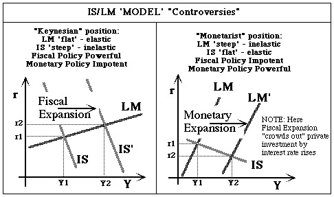
Your experiments with the IS/LM model should clearly show that the effectiveness
of Fiscal and Monetary Policies in governing (managing) the circular flow
of income depend on the slopes of the IS and LM curves.
If the IS curve is steep - then Monetary Policy will not
be very effective in managing income, but will only be succesful in managing
the interest rate.
On the other hand, if the IS curve is relatively flat, then Monetary
Policy will be effective in managing the levels of national income. The
effectiveness of Monetary Policy in governing levels of national income
depends on how steep or flat the IS curve is.
If the LM curve is steep, then Fiscal Policy (shifting the IS
curve) will mostly affect the interest rate and have little effect on national
income - the crowding out effect will be nearly 100% - attempts
to increase income with fiscal expansion will simply increase the interest
rate and have little or no effect on income, as a result of the government
spending crowding out private spending. Crowding out happens because the
government spending must be borrowed from the private sector, raising interest
rates and discouraging private spending, and, in the limit, means that the multiplier will be close to 0.
If the LM curve is flat, then Fiscal Policy will be powerful
in determining national income, and will have little effect on the interest
rate - there will be little crowding out.
Slopes of the IS and LM Curves:
The IS curve depends on the sensitivity (responsiveness) of aggregate
demand to changes in the rate of interest. It will be flatter the more
responsive aggregate demand (the expenditure loop of the CFoI) is to changes
in the interest rate. On the other hand, if aggregate demand (consumption
plus investment) mostly depend on the current state of the economy and
feelings or expectations about future incomes and spending (growth), then
interest rates may be relatively unimportant in determining aggregate demand,
and the IS curve will be steep.
The LM curve depends on the sensitivity (responsiveness) of money
demand to income - the more responsive the demand for money is to income
changes, the steeper is the LM curve. It is also the case that the more
responsive the demand for money is to interest rates, (the more elastic
the demand for money w.r.t interest rates) the flatter is the LM curve.
Managing the Economy
Scenario 1 - the classic Depression
-
If investors are "shy" of investing in expanded capacity because they are
unsure about the growth prospects for the economy rather than deterred
by the level of interest rates, the IS curve will tend to be steep (Keynes
referred to the "animal spirits" of business leaders being more important
to investment decisions than the rate of interest).
-
If, at the same time, the economy is stuck in a depressed state with consumers
tending to save more in the face of uncertainty about the future, hence
not increasing the demand for money much as incomes grow, then the LM
curve will tend to be flat.
-
If, in addition, the financial markets are following traditional patterns
of "portfolio management", seeking security and reliability from financial
and physical assets rather than "quick" profit or capital gain, then the
demand for (speculative or idle) balances will be insensitive to interest
rate changes and the LM curve will be flat
This is the story (approximately) for the Great Depression, and much of
the 50s and early 60s - power to Fiscal Policy and Money does not matter
much. If you want to get out of a 1930s type depression, then the Keynesian
solution of demand management works- kick start the depressed economy through
increased government spending over and above taxation receipts.
Scenario 2 - the more modern economy
-
If interest rates are important to investment decisions, then the IS
curve will tend to be flatter.
-
If incomes are expected to grow and personal savings are largely pre-determined
through current income levels (through mortgages, insurance premiums and
pension contributions), then increases in incomes may well be associated
with substantial increases in demand for money - as discretionary incomes
increase. So the LM curve will be steeper since increased demands
for money against a fixed supply will increase the interest rate.
-
As financial markets become more sophisticated and communications make
transactions faster and cheaper, and as the volumes of cash financial institutions
have to deal with increase, so financial portfolio management by large
companies may become more interest sensitive, making the LM curve steeper.
These developments during the seventies may well have made the economy
more sensitive to monetary management and correspondingly less sensitive
to fiscal policy. Power shifts towards Monetary Policy and away
from Fiscal Policy.
Effect of inflation: Notice, if there is inflation in
the economy, then this will reduce the value of money in terms of its purchasing
power, which will mean that more money is required to finance any given
level of transactions or level of real national income. This means that
the supply of money in real terms is reduced, shifting the LM curve to
the left, increasing interest rates and reducing the level of national
income.
Inflation will thus tend to reduce income and increase unemployment
- so long as monetary policy is kept reasonably tight. Overheating (expanding)
the economy will, in these conditions, generate stagflation (both
inflation and increased unemployment) - the typical economic condition
in the UK during the 1970s.
Modern Managment of the Economy
In the past, both monetary and fiscal policies have been used to try
and manage the economy so as to avoid both depressions and overheating
booms. However:
-
The information on the current state of the economy is always
out of date, so there is a tendency for economic managers to pull either
policy lever (Fiscal or Monetary) in response to past conditions, rather
than current conditions;
-
the time lags between pulling on either the monetary or the fiscal
levers and their effects on the economy are substantial and also variable.
It is this point which gives Monetary Policy an advantage - it can be changed
more frequently and easily than Fiscal Policy, where changes in tax rates
and schedules and changes in government spending take longer and more effort;
-
the structure of the economy - crudely summarised as the slopes
of the IS and LM curves - is always uncertain - so the balance between
effective monetary and fiscal policy is also uncertain;
-
Furthermore, the responses of the economy will depend very much on expections
about
the future, and also on its recent history (which conditions business and
consumption/savings responses). If the experience has been one of booms
and busts, then it is natural to expect people to expect the future to
be the same and respond accordingly.
All of these conditions make proactive management of the economic
cycle extremely difficult, if not impossible. In principle, it might seem
to be possible to expand the economy as it trys to move into a recession
and contract it as it begins to overheat - a counter-cylical policy as
a judicious mix of fiscal and monetary policies. In practice, however,
it is just as likely that such attempts will result in exacerbating the
cycle because of the near inevitability of getting the timing wrong - making
the recessions worse and the booms worse - rather than counteracting the
cycle.
Thus, the prudent approach to managing the economy is now thought to
be to keep a steady hand on both fiscal and monetary levers, and make as
much use as possible of automatic stabilisers.
Automatic stabilisers are those elements of government spending and
taxation which tend to operate counter-cyclically on their own, automatically
- government spending which tends to increase as the economy moves into
recession (like social security, unemployment benefit and employment policies)
and vice versa ; and taxes which tend to increase as incomes and
employment increase, and vice versa.
_____________________________________________________________________________________________________________________________
5. Aggregate Supply and Aggregate Demand (a cautionary note)
Aggregate Demand: We have already seen this concept in the Circular
Flow of Income. The total (aggregate) demand facing an economy is composed
of Consumption (C), Investment (I), Government spending (G), Exports (X)
minus Imports (IM). These are the flows of spending facing the firms in
the economy, which generate the national income, and the ability to pay
taxes (T) and to save (S).
Aggregate Supply refers to the responsiveness of the economy
in producing additional output and thus income to meet this demand. This responsiveness, however,
is not well understood. In general, the greater the demands placed on the
economy, the greater will be the supply, up to the point of full capacity
of the economy - or 'full employment' (unemployment levels low, since there will always be some unemployment as people change jobs and switch careers etc.)
But, the capacity of the economy depends on:
-
the size, skills and experience of the working population (Human capital)
-
the amount and quality of the capital plant and equipment etc. these people
have to work with (Physical Capital)
-
the skills of management in organising the people with the capital (as
well as the land) to produce output (Social Capital)
-
the productivity of capital and labour in producing output (the quality of the various capitals)
Each of these ingredients of the economy's capacity will change through
time. The greater the pressure on an economy's capacity limits, the stronger
the incentives to increase the capacity - frequently through investment
in peoples' skills and/or in the capital plant and equipment they have
to work with. Investment is also frequently associated with improved management
and productivity (generally reckoned to be improving at about 2%
per year, though not recently in the UK or the US).
If an economy does not typically run up against its capacity constraints,
then the incentives to increase and improve capacity will be weaker. Thus,
some inflationary pressure seems necessary to produce incentives for the
economy to improve and extend its capacity.
However, increases in aggregate demand seldom occur across the whole
spectrum of the components. Some sectors will experience faster growing
demand than others, encouraging a re-structuring of the economy (a reallocation
of resources from the declining sectors to the growing sectors), and thus
altering the aggregate supply curve. This re-structuring necessarily involves
price signals - those faster growing sectors exhibit tendencies
for their prices, wages and returns to increase faster than eleswhere in
the economy, and vice versa.
The resulting inflationary pressure of "excess demand" (aggregate
demand greater than aggregate supply) will be uneven, and pure
inflation
(equal proportional changes in all prices and returns) will almosr
never happen
through real demand pressures on the economy. As a consequence, the
actual
responsiveness of aggregate supply to increases in aggregate demand
will
depend critically on where the demand pressure is exerted.
Aggregate Demand and Aggregate Supply with respect to the Price Level
Notwithstanding these observations, many textbooks and commentators
use the notions of Aggregate Demand and Aggregate Supply with respect
to (w.r.t.) the Price Level to illustrate and explain macroeconomic
developments. Their diagrams are as follows:
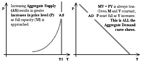
The AS curve w.r.t the Price Level is generally assumed to become
increasingly vertical as the economy approaches its capacity limit (otherwise
known as full employment - Yf). The superficial logic is that the
closer the economy is to full capacity, the more likely it is that additional
demands will generate increase in prices (inflation) rather than increases
in real output and income.
However, as noted above, this is likely to depend critically on the
way in which demand pressure is exerted, and also on the general expectations
of
those involved (the business community) on the likely persistance of these
pressures. For example, if these commerical concerns expect the emergence
of inflationary pressures to result in a contraction of the economy (as
macroeconomic policy tightens), then there will be less incentive to invest
for future growth, and the AS curve will be steeper (more likely to result
in price increases). On the other hand, if businesses expect that inflation
will be controlled, and the economy managed to generate more or less steady
growth, then demand pressure resulting in inflationary pressure might well
be interpreted as a sign of continued further growth - triggering increases
in productive capacity and supply. In other words, the notion of
a reliable AS curve is a figment of imagination - in practice, any such
simplification will depend critically on the context and circumstance of
the economy, and on expectations about the future. This does not
seem a very sensible simplification to me - it all depends!
In the limit, some extremists argue that the AS curve is always vertical
at the full employment level. There is NO supply response at the
aggregate level to increased demand pressure (expressed as pressure to
increase the price level). This argument is based on the microeconomic
theory that supply only responds to relative prices, not to the
absolute level of any price. In a pure inflation (uniform
changes in all prices equal to the change in the overall price level) the
relative prices (each price relative to others, do not change -
so there will be no supply response to a change in the price level.
In this case, demand expansion will only result in inflation and
never
in an increase in real income and employment. Trying to boost the
economy with fiscal expansion, in this case, will simply generate inflation.
This is all true for PURE inflation - and the AS curve would be vertical
under these conditions - BUT these condtions NEVER happen - they are a
figment of the theorist's imagination. In practice, inflationary
pressures happen in some bits of the economy more than others, some prices
keep pace with or exceed the general inflation rate and other do not.
The AD curve, on the other hand, ONLY shows the general macroeconomic
relationship between real income (Y) and the price level (P). This is NOT
THE SAME THING as the microeconomic relationship between quantities demanded
and specific (relative) prices. An increase in P means that ALL PRICES
AND RETURNS increase at once. This means that RELATIVE PRICES DO NOT CHANGE.
The microeconomic demand curve shows the response to a change in the price
of one good or service (or factor of production) relative to all others.
If relative prices do not change, then microeconomic demand quantities
DO NOT CHANGE EITHER.
So, the AD curve DOES NOT SHOW THIS MICROECONOMIC RELATIONSHIP. All
it shows is the various possible combinations of P and Y which could go
to make up the total nominal demand in the economy:- P*Y, given a
fixed money supply and fixed velocity of circulation. Thus, increases in
AD are shown by shifts
of the AD curve to the right and vice
versa. These shifts could arise because of:
-
increases in the money supply (monetary expansion - equivalent to reductions
in the interest rate);
-
expansionary fiscal policy;
-
increases in autonomous (not government controlled) aggregate demand (increases
in investment (I) or net trade (X - IM) or reductions in savings and associated
increases in consumption).
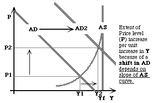
Any of these increases in AD could result in either an increase in the
price level (P) or an increase in real income and output (Y), or both,
as shown in the AS/AD diagram. So what do we learn from this? Not very
much at all, since the answer to what will actually happen is that it all
depends on what sort of demand increase we are talking about, and hence
what sort of shape the relevant AS curve looks like. IN SHORT, I
DO NOT FIND THIS ANALYSIS EITHER VERY CONVINCING OR VERY HELPFUL in understanding
how the economy works. Do you? Comments
and questions to DRH.
_____________________________________________________________________________________________________________________________
6. The Phillips Curve
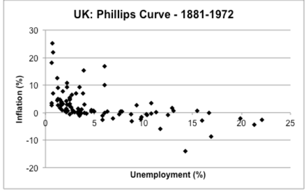
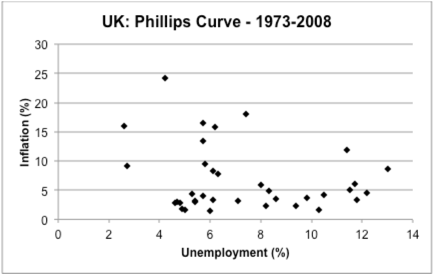
The ideas underying the Aggregate supply curve lead to a notion of the Phillips Curve - a trade-off between Inflation (as the general (average) rate of change of prices in the economy) and Unemployment. So called after A W Phillips, who identified an apparent statistical relationship between inflation and unemployment. Economics online has a good account of this relationship, and its place in current macroeconomic thinking.
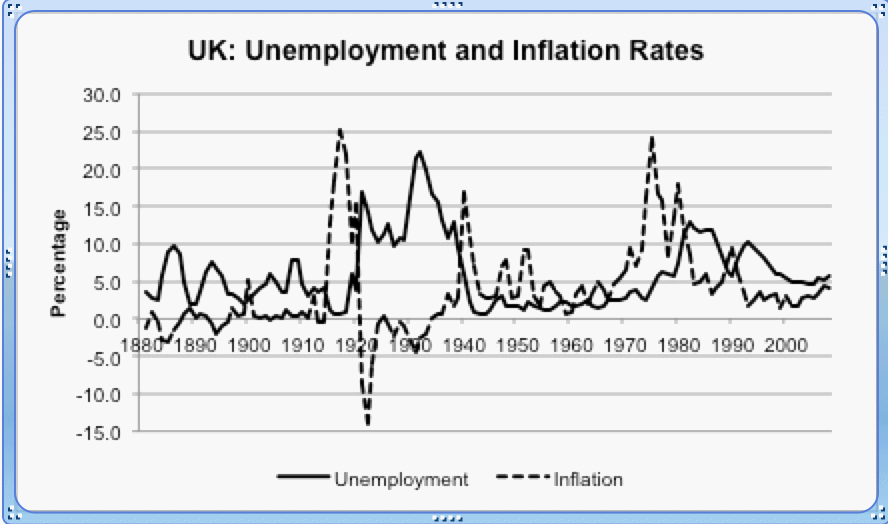
Sources: Unemployment statistics from 1881 to the present day
(1881-1994):
http://www.ons.gov.uk/ons/rel/lms/labour-market-trends--discontinued-/january-1996/index.html
& ILO: http://laborsta.ilo.org/STP/guest
Inflation Consumer Price Inflation since 1750: www.ons.gov.uk/.../consumer-price-inflation-since-1750.pdf
[A useful page for historical UK Inflation rates - back to 1751]
 _____________________________________________________________________________________________________________________________
For an excellent data visualisation and data source for world economies macro conditions and development: see IMF Datamapper.  (Reconcilliation of these data with data for farming alone is slightly problematic)


The IS curve shows
the equilibrium relationships between the rate of interest (established
in the money market) with the level of national income,
assuming
that
the remaining injections and withdrawals (G, T, X and IM) stay as before.
If these other (exogenous) injections and withdrawals
change,
then the IS curve itself will shift.
![]() slopes
downwards because lower
slopes
downwards because lower![]() interest
rates (r down) encourages investment and consumption and thus increases
interest
rates (r down) encourages investment and consumption and thus increases![]() national
income (Y). It thus represents the combinations of r and Y which are consistent
with equilibrium in the goods and services markets (the circular flow
of income). Note this. The CFoI is, in effect, a description
of equilibrium in the markets for goods and services (and factors of production)
-equilibrium in the 'real' (non money) part of the economy.
national
income (Y). It thus represents the combinations of r and Y which are consistent
with equilibrium in the goods and services markets (the circular flow
of income). Note this. The CFoI is, in effect, a description
of equilibrium in the markets for goods and services (and factors of production)
-equilibrium in the 'real' (non money) part of the economy.
The LM curve shows
all those combinations of Y and r which are consistent with an equilibrium
in the Money Market (given a fixed money supply and a constant velocity
of circulation)


 _____________________________________________________________________________________________________________________________