ACE 2006: Microeconomics of Supply

Economical Simplification of a single Business or Firm of any sort - the logic of competitive supply: The following is an explanation of the implications of competitive survival of firms, NOT a management prescription of how to manage such firms.

What happens to total costs as production levels increase, ceteris paribus? The ONLY things which we are changing in this analysis are the level of output (production) of the firm (and thus the level of inputs and resources that are needed to produce more output). The costs of the inputs per unit are held fixed and constant. The technology available is fixed. The quality and productivity of the inputs are given and known, and unchanging. The quality of the product is fixed.

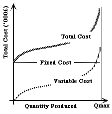Summary: Fixed costs are those costs (including all relevant opportunity costs) which do not vary as the quantity produced varies. Variable costs are those costs which do vary as production quantities change (increase as output is increased). Total costs equal fixed costs plus variable costs. The general shape will look pretty much like this, for any production process we care to think of.

Fixed Costs - sometimes considered to be equivalent to the costs of the factors of production: land, labour, management and capital plant and equipment etc. - the resources needed to be in production at all.
Variable Costs - sometimes considered to be equivalent to the costs of the purchased inputs (fuel, raw materials, packaging materials etc.) No one can produce something for nothing - variable cost, and total cost, will always increase as we increase production, supply, delivery - though may increase only a very little over some part of the business's output or throughput possibility range
However, the distinction between fixed and variable costs depends critically on the particular and specifc conditions and circumstances of the firm in question. The precise details of these specific (and highly differentiated) conditions do not need to concern us here. The general principles still apply, whatever the precise fixed or variable classification of particular costs. The specific classification of costs is not fundamentally important.

Unit Costs - costs per unit produced:

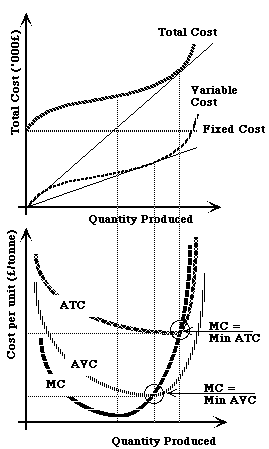Summary of Costs per unit produced:

Average Total Costs (total costs ÷ quantity produced) is shown by the slope of a line from the origin to any point on the total cost curve. ATC is therefore "U" shaped, with a minimum where the origin line is tangential to the total cost curve.
Average Variable Cost (AVC) is defined in exactly the same way (as total variable costs ÷ quantity produced), and exhibits the same "U" shape.
Marginal cost (the cost of an extra or additional unit of output) is the slope of the total cost curve itself
MC is at a minimum where the total cost curve is flattest, where its slope is least.
For the quantity at which average cost is at a minimum, average cost is equal to marginal cost. The marginal cost curve cuts the average cost curve from below, at the average cost curve's minimum point. This has to be true by definition. Average cost at its minimum is the slope of the tangent from the origin to the total cost cost curve. The tangent to the total cost curve has the same slope at that point as the slope of the total cost curve, which is the marginal cost at that point.
These diagrams assume that the manager(s) of the firm are as efficient as they can be in making and implimenting the decisions to change output levels. They are effective in keeping costs as low as possible consistent with health, safety and product integrity. In short, they assume effective business managment and operation.

Maximising Profits - stylised illustration of the firms cost curves:

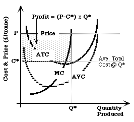To maximise profits ( = total revenues minus total costs): produce at that output level at which marginal cost equals marginal revenue. So long as the MC curve is rising, this will mean that all previous units of output cost less to produce than they earn in revenue, and any greater level of output will cost more to produce than it earns in revenue.
In a competitive industry (many other competing firms) the price is set by the market - firms in a competitive market are Price Takers: there is no sense in charging less than the other firms, because this firm cannot produce enough to satisfy the whole market, and if it trys to charge more, it loses sales to other competing firms.
In this competitive case, Price = Marginal Revenue (MR) (the addition to total revenue consequent on the sale of one extra unit). Hence, profit maximisation involves producing at the quantity for which MC = MR = Price. If the market price is P, then the profit maximising output level is Q*, at which point MC = MR.
At this point, Average cost = C*, so that total cost = C* x Q*, while total revenues = P x Q*. So, Profit = total revenues minus total costs = (P - C*)x Q* = the shaded area.
This profit is Pure (Economic) Profit - since the total costs include all opportunity costs, the excess of revenues over total costs is pure or economic profit over and above the returns necessary to cover all costs. NOTICE - this Price = MC rule is the logical outcome of a firm's competitive behaviour, NOT a prescription for the effective management of the firm.

If this firm is making pure profit, then other firms will be attracted into this industry to produce this product. As they do, so total market supply will increase, and the market price will fall (and, quite probably, firm costs will increase as firms try and obtain more resources and purchase more inputs, driving up the costs). When will this competitive market be in equilibrium?

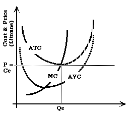When Price = MC = Min ATC (at Ce in this diagram) with no pure profits to encourage firms to expand or enter the industry, and enough to cover all costs, including opportunity costs. Each of the firms make just enough of a return to be willing to stay in the business rather than doing something else. The return that is just enough is the return which covers all of the costs, cash costs and opportunity costs. The opportunity costs measure how much each firm could earn if it moved its land, labour, capital and management into some other business or occupation. So long as each earns at least this return, each will be content to stay in this business indefinitely. If prices fall below this level, firms will leave the industry as the opportunity arises, and supplies will fall, and prices will start to rise again back to the equilibrium level.

Industry Supply - depends on:

each firms individual response to price changes
the change in the number of firms in the industry (product producing sector)
whether the situation is supposed to be Long or Short Run

Long Run: all factors of production and all production inputs considered to be Variable - can be changed by the firms in response to changes in their economic environment.
Short Run: - at least some factors of production and inputs are considered to be fixed at their current levels - cannot be changed in response to changing signals.

greater scope for responses in the Long run

1. Firm's response to price changes:

represented by the firm's marginal cost curve. For a firm in a competitive industry or sector, profit maximising means producing where price = marginal cost. Hence, as price changes, so firm output will change according to the MC curve.
Long Run Marginal Cost curves will generally be flatter - more elastic - than Short Run marginal cost curves.
For firms in a competitive industry (many competing firms), any one single firm's changes in output, and hence changes in demands for inputs and resources, will NOT significantly affect the costs per unit of each of these inputs and resources. Hence, marginal cost (and all other cost curves) for the firm assume that the cost per unit of inputs and resources is fixed and given. Marginal cost curves slope upwards because each extra unit of output requires more physical units of input and resource to produce - not because the prices of these inputs increases. NOTE - if this is not the case, then the firms were not operating efficiently in the first place - they could have produced more and earned more than they were doing.

2. Industry response to price changes (caused by shifts in demand for the products):

In the Short Run - the industry supply curve can be thought of as the sum of all the individual firms marginal cost curves.

BUT, there is one important caveat to this notion:

If all firms increase their outputs up their marginal cost curves, they are all demanding more inputs to produce the extra output.
This increased demand for inputs (shifting input demand curves to the right) will tend to increase the price (unit cost) of the inputs.
This increase in the cost of inputs will shift the marginal cost curves upwards.

Hence, the Short Run Industry Supply Curve (SRS) will tend to be Steeper (more inelastic) than the individual firms marginal cost curves, because their collective demand for inputs will tend to change the prices of these inputs.

In the Long Run - increased demand for the industry products will tend to increase the price, thus increasing the profits earned by each firm in the industry. More firms will be attracted into the sector, shifting the SRS to the right, increasing industry output and reducing prices again.
The outcome is illustrated in the following diagram. Start at an equilibrium position of Pe, with firms producing qe, all making normal profits (that is, covering all their costs including their opportunity costs) and with the sum total indistry output at Qe.
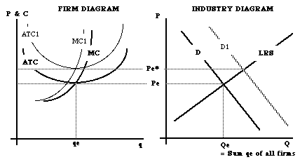Now suppose that demand shifts right to D1. Initially, each existing firm increases output up its own MC curve, and makes pure profits. New firms are attracted into the industry, increasing industry output and damping down the initial price increase. Increasing output increases the costs of inputs which shifts cost curves upwards to MC1 and ATC1. The new long run equilibrium results when firms are once again only making normal profit (price Pe* = ATC1 = MC1), just covering all costs at their new level.
The Industry long run supply curve (LRS) traces out the increase in output resulting from the shift in demand.
Key Factors affecting the elasticity of supply

It will always take time for the full supply response to a demand change to materialise - long run elasticities more elastic than short run. Over and above this general condition:

Flexibility of production systems and processes - the more flexible, the more elastic supply;
The more permanent the shift in demand is expected to be, the more likely it is that firms will take long run decisions and that new firms will become established - so the more elastic the supply response will be.
The more industry or sector specific are the inputs and resources used, and the more limited they are in supply, the greater will be the cost increase associated with industry expansion, and the less elastic will be the industry supply response; (e.g. - agriculture, with the requirement for land, which is limited in total supply).

Imperfect Competition: the key difference between perfect competition and imperfect competition is the nature of the demand facing the firm. -

perfect competitors are Price Takers - cannot set or affect the market price on their own;
imperfect competitors are Price Setters - they can set their own prices, and their sales levels affect the prices they can charge.

Imperfect competitors face downward sloping demand curves, rather than the perfectly elastic (horizontal) demand curves which facce each FIRM in perfect competition.
So, for imperfect competition, Price DOES NOT equal Marginal Revenue (MR) - the additional revenue earned by imperfect competitors from the sale of an extra unit of production requires that the price charged for all sales has also to be reduced - the Marginal Revenue curve is therefore steeper (more inelastic) than the demand curve.
For a linear demand curve, the MR curve will be twice as steep as the demand curve (beginning at the same price on the vertical axis as the demand curve, but intersecting the horizontal (quantity) axis at half the quantity of the demand curve

Monopolistic Competition: - differentiate their products from those of their competitors (advertising, brand loyalty etc.), but are vulnerable to competition from rival firms for market shares.

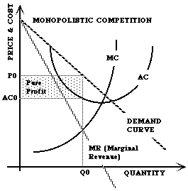Profit Maximising means produce at quantity for which MR = MC.
Set price for this quantity (Q0) according to consumers willingness to pay (the demand curve price for this quantity - P0
Cost of producing this quantity (Q0) is AC0 per unit, so profit = (p0 - AC0) x Q0; the shaded area.
So, more firms will try and enter this industry
with the effect that the demand curve and MR curve for this firm will SHIFT to the left as new entrants take market share
Equilibrium in this Monopolistic Competition sector will occur when there are no pure profits left to attract new entrants
No Pure Profits when, and only when, the Demand Curve shifts far enough to the left to lie at a TANGENT to the AC curve - then Price is set so as to equal AC.
At this production (sales) point, MC will also equal MR - profit maximising with no pure profits.

Pure Monopoly: The same as Monopolistic Competition EXCEPT that new firms CANNOT enter the market to errode this firms market share.
The first diagram above, from Monopolistic Competition applies to Monopolists.
Reasons for Pure Monopoly - single supplier to whole market:

Natural Monopoly: production and supply conditions such that there is only room for one supplier from the whole market - costs are such that one firm can supply the total market more efficiently (lower costs) than a collection of firms (e.g. gas, electricity, railways etc.)
Patent rights over technologies - giving single firm temporary advantage
Monopoly Property Rights over necessary raw materials
Predatory business practices and artificial barriers to entry of other potential competitors

1 and 2 are probably justifiable reasons for a monopoly - 3 and 4 are not, and are typically outlawed, or at least restrained (by patent laws, etc.).
But Monopolists do not always make pure profits because:

Market is not large enough to allow monopolist to exploit cost advantage - railways in early days.
Market shrinks because of substitutes (e.g. road and air for rail) - note: existence of close substitutes will make demand facing monopolist more elastic - bringing demand and MR curves closer together and reducing scope for pure profits.
Costs increase (cost curves rise) because:

suppliers and labour force also have more market power against a single user
management performance falls through lack of competitive spur to do better

Natural Monopolies are sensible from an economic point of view - but require Regulation by Government to ensure that consumers and users are not ripped off.
Major Problems for Regulators:

Control over monoplists costs - how to ensure efficient production and operation?
Setting socially acceptable prices - how to set prices to users so as to cover legitimate costs but not result in over-supply (costs higher than willingness to pay)?

So: Competition ensures that consumers and users benefit from the lowest prices possible (consistent with producers earning sufficient incomes to persuade them to stay in the business, and competition encourages firms (producers) to stay as efficient as possible, encouraging innovation and adaptation in the interests of increasing value and improving efficiency. Nevertheless, it is an uncomfortable business environment, and we might expect producers to try and protect their own markets if at all possible.

Back to Index