AEF811: MACROECONOMICS: THE BASICS
Note: to use as a dictionary of terms - use "find" in your
browser menu bar.
Managing in and with markets requires some knowledge of the basic
Macroeconomic relationships - concerning interest rates, income growth
rates, exchange rates, unemployment rates etc. These notes are a
very brief outline of the major elements of Macroeconomics. For those
who would like a more extended treatment, see any introductory textbook
of economics, or try my first year undergraduate macro
economics course notes.
CONTENTS:
Comments,
questions and suggestions??
-
The Link between Microeconomics and Macroeconomics - General
Equilibrium in all markets
-
Macroeconomic Basics - the Circular Flow of Income (CFoI),
with Government and Fiscal Policy
-
Macroeconomics of Money Money Markets, Financial Markets
and Capital Markets - and Monetary Policy
-
Macroeconomics of Money with the CFoI( IS/LM): Monetary
and Fiscal Policy to achieve Macroeconomic equilibrium (low Unemployment
and low Inflation)
-
Macroeconomics of International Trade - The Forex market
-
MacroEconomic Management:
1. The Link between Microeconomics and
Macroeconomics - General Equilibrium in all markets and Value Added
The Market system works through specialisation and trade:
People, communities, regions and countries are better off specialising
in production and trading the products with neighbours than they would
be if they tried to be completely self-sufficient. If this were not
the case, markets would not exist.
Specialisation and Trade relies on people and their businesses exploiting
their comparative advantage - specialising their productive activities
in those areas and products for which they are best able, relative
to all the other things which they might do instead. Their opportunity
costs should then be less than the returns they can earn doing their present
things, and they will make a positive return as a consequence.
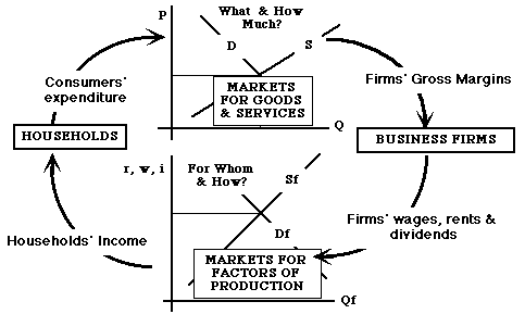
The general picture of interacting markets - the circular flow of income:
-
Households own the factors of production (land - including
raw materials, labour, management and physical capital).
-
Note - capital here means physical capital - plant, equipment, buildings
and machinery etc. (c.f. financial and money markets below)
-
Households rent these factors to firms, in return for income:
land rents; capital interest and dividend payments, and equity appreciation
(capital gains); wages and salaries.
-
Factor ownership provides income which fuels consumption and demand in
the goods and services markets
-
Firms rent the factors of production from households according to their
demands for these factors, which is derived from the demands for
the final goods and services
-
Factor markets operate so as to encourage the owners of land, labour, manaement
and capital to rent out the services of the factors to the highest bidder
-
Firms add value to their own purchases of inputs and raw materials.
They earn gross margins (total revenues minus cash input costs [fuel,
power, packaging etc.] which is the value added to these inputs.
The Gross margin, or added value, or gross product
(each term means essentially the same thing for our purposes) is the income
available to the fixed factors - land, labour, management and capital.
-
In equilibrium, these returns will be normal profits - each firm earning
sufficient to cover the opportunity costs of the factors of production
which they employ.
[Note: profits in the everyday sense are, typically, just the
returns to capital - the earnings of the firms which are left after all
other legitimate costs (including labour and management costs) have been
deducted. For self-employed family businesses, taxable profits will
include the returns to the owners own labour and management, as well as
returns to the owners land and capital, less allowable expenses in servicing
mortgages, loans and debts.]
The UK food chain illustrates the outcome of this circular flow of income.
Agricultural and Food Chain, UK, 2000
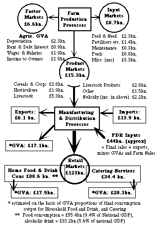 Farms produce £15.3 bn. of output, of which £8.7bn. is spent
on purchased inputs, leaving £6.6bn. as the gross product (gross
margin) or returns to the factors of production (land, labour, management
and capital).
Farms produce £15.3 bn. of output, of which £8.7bn. is spent
on purchased inputs, leaving £6.6bn. as the gross product (gross
margin) or returns to the factors of production (land, labour, management
and capital).
-
The farm sector generates incomes to all those with a direct interest in
farming - the labour, owners of the capital (including the banks and their
shareholders), the owners of the land, and the managers and farmers themselves.
-
Likewise, the input supply industries also process their own inputs, using
their own factors of production, producing their outputs (purchased by
the farm sector) and generating their own incomes to land (including natural
resources), labour, management and capital.
-
Farm Output, in turn, is further processed by the Processing, Distribution
and Retailing (PDR) sectors to generate both incomes to their own factors,
and also the final output purchased by the final consumers.
-
Thus, the final consumption figure (£123 bn.) represents the
cumulative total of all values added throughout the food chain,
and hence represents the total cumulative income earned by all those
engaged, both directly and indirectly, in the food chain.
-
Note that imports generate incomes in other countries rather than the UK,
while exports generate incomes in the UK.
Measurement Issues:
-
Each of these flows (measured in £ bn.) represents a large collection
of individual trades (prices times quantities): P
x Q
-
Flows change through time because both prices and quantities change: P1
x Q1 different from P2 x Q2
-
Comparison between different years (periods) compares both price and quantity
changes
-
Prices represent that rates at which quantities of one good or service
are exchanged for other goods and services - including the services of
factors of production (land, labour, management and capital), whose prices
are rents, wages and salaries, and rates of return to capital.
-
With prices set at some given, fixed level: quantities then
represent real income and real output of goods and services
- the actual quantities of factor services which can be traded for the
purchase of actual quantities of goods and services - the purchasing power
of each good or service in terms of all other goods and services.
-
To measure these real quantities, prices (wages, rents etc.
as well as prices of goods and services) have to be fixed at some given
level. - Pf. - constant prices
-
Comparison of Pf x Q1 with Pf x Q2 then shows the changes in quantities
between Q1 and Q2.
-
Also, comparison between Pf x Q1 and P1 x Q1 shows the difference in prices
between the fixed, constant, prices and those ruling in period 1.
-
Notice - simply fixing the price of ONE good (say for fertiliser), allows
the actual physical quantities of fertiliser used by farms between years
to be measured, but does NOT allow the measurement of the purchasing power
of this fertiliser - to measure the purchasing power, we need to
fix
all prices at some constant level.
Back to Contents.
2. Macroeconomic Basics
- the Circular Flow of Income (CFoI)
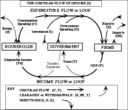
Simplify the whole economy as an interaction between Consumers (households),
Producers (firms), and Government. NOTE: This is a circular
flow of INCOME (and spending) - although measured and identified in money
terms, it is the livings (income and spending) - the real purchasing
power of the money - which is important here. Always refer to the
flow as an INCOME flow and not a flow of money.
Notice, too, that Income (GDP) is typically related to the level of
employment and unemployment - the lower the level of GDP relative to its
trend, see below, the higher the level of unemployment.
-
Consumption (C) is spending on goods and services for final use
(consumption) during this period.
-
Investment (I) - an injection into the CFoI - is the
purchase of actual physical capital (equipment etc.), or the improvement
of peoples skills and expertise - final spending on things which are intended
to increase income levels in future periods rather than this one.
[Please Note: Firms are responsible for most of this investment,
not governments, though some government spending is investment for future
periods rather than spending on current (this year's) goods and services]
-
Saving (S) is just and only income which is NOT spent on final goods
and services. (= Yd - C) - a withdrawal from the CFoI. [Please
Note: Investment spending is matched with Savings through the
financial
and money markets (see below), which are separate from this
Circular Flow of INCOME picture of the economy]
-
Government Spending (G) is ONLY spending on final goods and services
(wages and salaries, paper, power, building maintenance and improvement
etc.) used up in this period or intended for use in future periods (includes
any government investment) - an injection into the CFoI
-
The other (major) part of total government expenditure is Transfer Payments:
social security, unemployment benefit, public (national) pension payments
etc. which simply add directly to the recipients incomes, and which
are not paid in return for actual services.
-
Taxes are the government reciepts - actually also raised on the
spending loop (VAT, excise duties), as well as on income streams (income
and corporation taxes) - T is best thought of as total taxes minus
transfer payments - a withdrawal from the CFoI
-
Exports of goods and services provide income for firms, and also
measure this part of total output of the economy - an injection
into the CFoI
-
Imports of goods and services leak income out of the national (domestic)
flow of income - a withdrawal from the CFoI
-
Total Expenditure equals Output (C + I + G + X - IM) equals Income (called
Gross Domestic Product) (Y) which equals Disposable Income (Yd) plus Taxes.
NOTE: Necessary Accounting equality (Total Expenditure = Income)
over any one period (one year) does not necessarily imply equilibrium.
If Expenditure is growing, then so too will income - and both will be larger
in the next period. If income is falling, then spending will also
fall, and both will be smaller next period.
Distinguish between
-
trend growth (improvement in technology and productivity (outputs per unit
inputs)) typically about 2.5 - 3.5% per year
-
cyclical growth (or decline) round the trend growth - booms (strongly positive
growth rates) and recessions (slower growth rates) or depressions (negative
growth rates).
Equilibrium Process of the CFoI.
-
Increasing Injections (G, I, X) and/or reductions
in Withdrawals (T, S, IM) will increase the CFoI (increasing
income and output (expenditures) and vice versa.
-
Multiplier process - increasing an injection (for instance) increases
income, which then leads to further increases in spending and resulting
income
-
until income levels have risen sufficiently that new levels of withdrawals
equal the new level of injections (increasing incomes tend to lead to increased
savings, taxes and imports). Y (GDP) will not be in equilibrium
until
resulting Withdrawals balance Injections
Fiscal Policy as a stabiliser of economic cycles:
-
Government Fiscal Policy (the balance between G and T) can influence equilibrium
Income levels
-
Increase G (or reduce T) to counteract a recession
-
Reduce G (or increase T) to counteract an unsustainable boom (income growth
exceeding full capacity of the economy, which leads to inflation - see
below)
Capacity Limits:
-
Total Capacity of the economy to generate output and income depends on
the quantities of land, labour, management and capital plant and equipment
available
-
When all of these factors of production are fully employed, the economy
is operating at full capacity. Otherwise, there is unemployment -
the economy could produce more income and output.
-
Capacity can be increased by:
-
investment in capital plant and equipment - more
capital for production and output;
-
increase in the labour force participating in
the economy - more employment -> more output & income;
-
improvement in technology - more output &
income from the same amounts of labour and capital through technological
improvement - better quality and more productive capital;
-
improved productivity of labour - better skilled
and better organised labour increasing the amounts that can be produced
and the income that can be earned;
-
structural change- re-organisation of resources
among different firms with lower costs, improving management.
-
Fiscal Policy (G and T) can affect these capacity increasing
processes - so should be used with care and caution.
Money and CFoI (and Inflation)
-
National Income (GDP) = P x Y (a
grand sum of millions of price times quantity trades) - where
Y
is real income - in terms of purchasing power over all goods and
services, and P is the general price level (an index of all prices
in the economy)
-
Money (M) is the medium through which these trades
take place (notes, coins, and current accounts with banks)
-
Money is a STOCK which is exchanged between different
people and businesses as trades happen
-
The FLOW of money round the CFoI is given by M
x V, where V is the Velocity of Circulation - the number of times
any one £ changes hands in the course of 1 year.
-
MV = PY (the Quantity equation of exchange)
always holds - it is the only way of defining and measuring V.
-
If V is constant, then PY (nominal or current GDP, national
income) can only increase if M increases.
-
If Y is fixed by the Capacity Constraint - at Yf (full
employment national income), then any increase in MV will lead to an increase
in P - inflation.
Back to Contents.
3. Macroeconomics of
Money
Money is used both as a medium of exchange for transactions (active bank
balances) and also as a store of wealth (idle bank balanes).
 Demand
for and Supply of Money: The price of money is the interest rate
Demand
for and Supply of Money: The price of money is the interest rate
-
Demand for money (current account bank balances) depends on:
-
Income (especially for transactions or active balances)
-
Price (the interest rate) especially for idle balances - the higher the
interest rate, the greater the opportunity cost of holding wealth as money
rather than as financial or physical assets.
-
Money Supply is controlled by the Monetary Authority - the Bank of England
(BoE).
-
Monetary Policy is decided by the Monetary Policy Committe of the BoE,
with the objectve of controlling inflation
-
either through controlling the Supply of Money directly (which proves to
be rather difficult)
-
or by setting the base lending (interest) rate of the Bank of England to
the commercial banking system - the current system of Monetary policy.
(Setting the interest rate at a new level above r* will automatically result
in a contraction of the supply of money to match the reduced demand - since
the BoE, through its function as lender of last resort, implicitly sets
the supply of money to match its ruling interest rate)
Financial Markets -> the rate of interest
-
Rate of Interest = price of money:- the cost of getting more of it from
banks etc., or the opportunity cost of saving (= storing income as wealth,
by owning assets, from savings accounts (loans to other people and businesses)
up to land, buildings, and old master paintings)
-
Assets differ in terms of:
-
their Liquidity (how easily and cheaply they can be transformed
into a certain amount of money (for transactions).
-
their Rate of Return - how much they earn in annual interest payments
(and how much they will appreciate in value (capital gain). Higher
liquidity typically means lower rates of return.
-
The Rate of Return earned by any asset is fundamentally related to the
ratio of the current capital value of the asset (its price for outright
purchase now) to its annual return (i). In general, Present Value
of an asset = discounted sum of all future returns (annual payments or
Future Values), where the discount rate is the rate of interest.
-
The Internal Rate of Return (i) is that rate of interest which makes the
present value = the current market price for the asset
-
The higher the price (capital value), the lower the rate of return, and
vice versa (ceteris paribus)
-
The higher the rate of interest, the lower the Present value of assets
(their prices)
-
Rates of Return differ because:
-
differences between borrowing and lending rates = payment
for services (which could be charged for separately).
-
differences in the risks associated with each different asset. The
more risky, the higher the rate of return necessary to persuade people
to accept the risk. Differences in risk also account for differences
between banks borrowing and lending rates.
-
the value of money itself is not guaranteed - inflation happens.
Uncertainty about future inflation rates, and the extent to which any particular
assets annual returns will keep pace with inflation or not (the sensitivity
of returns to inflation), also affect the rate of return on assets.
-
In general: the rate of return on any asset i = r + u + p,
where i is the asset's rate of return in current or nominal terms:
r is the real interest rate (opportunity cost of money); u
is the risk premium for this asset; p is the expected rate of inflation.
[Note: physical assets also depreciate (wear out and become
obsolete), so their value diminishes over time - so their rate of return
has to include an allowance for depreciation (d).]
All these factors affect different assets and their rates of return (or
interest rates) differently. The financial markets are where
these differences are traded off with and against each other. So
long as these markets are competitive (no one person or business can affect
or partially control the supplies or demands for financial and physical
assets), then all these different interest rates will end up being closely
and reliably related to each other in an inter-related constellation
of interest rates. If one asset shows exceptional returns relative
to the others on offer in these markets, then investors will flock towards
the premium asset and away from the others. The price paid for the
premium asset will rise relative to the rest, and the return to be earned
as a percentage of the buying (aquisition) price will fall. The result
will be that the premium return (interest rate) disappears and comes back
into line with the other rates, given its risk and inflation characteristics.
Conclusion: a single interest rate is sufficient to represent
all the different interest rates exhibited in competitive financial markets,
which underly the Money market above.
Capital Markets:
The rate of interest also influences Savings and Investment - the balance
in the capital market for loanable (investment) funds
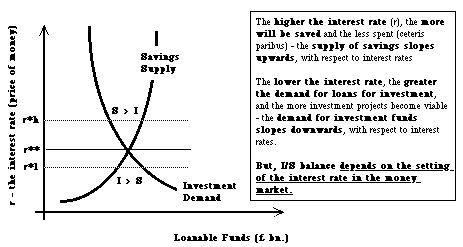 Notice:
If the interest rate (set in the money market) results in I > S, then there
will be a tendency for the level of National Income (Y) to grow - increasing
savings (shifting this ceteris paribusSavings supply curve to the
right as incomes increase) to match the additional investment. However,
increasing Y might also increase Imports and Taxes - so that the imbalance
between savings and investment might persist - offset by imbalances between
G and T, and between IM and X.
Notice:
If the interest rate (set in the money market) results in I > S, then there
will be a tendency for the level of National Income (Y) to grow - increasing
savings (shifting this ceteris paribusSavings supply curve to the
right as incomes increase) to match the additional investment. However,
increasing Y might also increase Imports and Taxes - so that the imbalance
between savings and investment might persist - offset by imbalances between
G and T, and between IM and X.
Back to Contents.
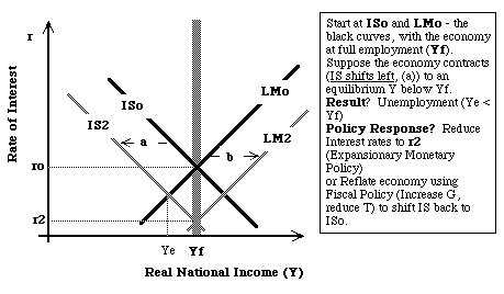
4. Macroeconomics of
Money with the CFoI( IS/LM)
Management of the Macroeconomy depends on achieving an appropriate balance
between the markets for goods and services (as represented by the CFoI)
and the money markets (as above.
It therefore depends on achieving an appropriate balance between the
two major levers of macroeconomic management: Fiscal Policy and Monetary
Policy.
The Key variables in this balance are the level of national income
(Y) and the rate of interest (r) - charted on the IS/LM diagram:
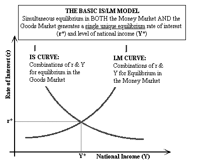 The IS curve
refers to the equilibrium levels of National Income in the markets for
goods and services (CFoI). Here, higher rates of interest are
associated with lower levels of spending (higher savings, lower investment,
lower levels of consumption) - so the IS curve slopes downwards. Note
the direction of causation: setting the interest rate determines
savings (withdrawals) and investment (injections), which then determines
the equilibrium level of national income.
The IS curve
refers to the equilibrium levels of National Income in the markets for
goods and services (CFoI). Here, higher rates of interest are
associated with lower levels of spending (higher savings, lower investment,
lower levels of consumption) - so the IS curve slopes downwards. Note
the direction of causation: setting the interest rate determines
savings (withdrawals) and investment (injections), which then determines
the equilibrium level of national income.
The LM curve refers to the equilibrium in the Money Markets
-
given
a fixed money supply. Here, higher levels of national income lead to
greater demand for money (for transactions), and hence higher rates of
interest (given a fixed money supply)- so the LM curve slopes upwards.
Note
the direction of causation (opposite from IS curve) - incomes drive the
demand for money, which then sets the interest rate if the supply of money
is fixed (or sets the supply of money if the interest rate is fixed)
Fiscal Policy affects the IS curve - expansionary (increase
G, reduce T) shifts IS right, and vice versa.
Monetary Policy affects the LM curve - expansionary (increasing
Ms, reducing interest rates) shifts LM right, and vice versa.
The relative effectiveness of Monetary and Fiscal Policies in influencing
Y (and thus employment) depends, therefore, on the slopes of the IS and
LM curves.
The steeper the LM curve, the greater the "crowding out" effect
of government spending - G increases increase interest rates which reduce
(crowd out) private spending.
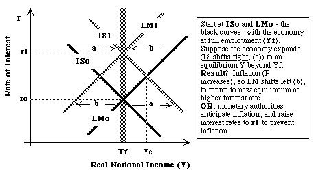
Inflation effects - If equilibrium Y* is greater than the full
capacity of the economy - there will be pressure on prices - leading to
inflation. Inflation reduces the value of the fixed Money Supply,
shifting LM left, raising interest rates and reducing Y* back towards
its full capacity level.
BoE MPC raising interest rates to limit inflation is the practical
counterpart of this effect - by rasing interest rates, the MPC effectively
holds the Money Supply constant in the face of increasing demand.
Back to Contents.
5. Macroeconomics of
International Trade
What, if anything, balances Imports with Exports in the CFoI?
The Foreign Exchange (Forex) market - where people and businesses
trade one currency for another.
-
Demand for sterling (= supply of forex) depends on exports
of goods and services, and on inward flows of investment funds from abroad
(capital inflows)
-
Supply of sterling (= demand for forex) depends on imports
of goods and services, and on outward flows of investment funds from the
UK to foreign countries (capital outflows)
-
Balance of Payments (BoP) records all these transactions:
-
Current Account (Exports vs. Imports)
-
balance of visible trade
-
balance of invisible trade (services, tourism travel etc.)
-
Capital Account (flows of investment (financial) funds into and
out of the country
-
Official Financing - change in the BoE forex reserves.
The 1996 UK situation:
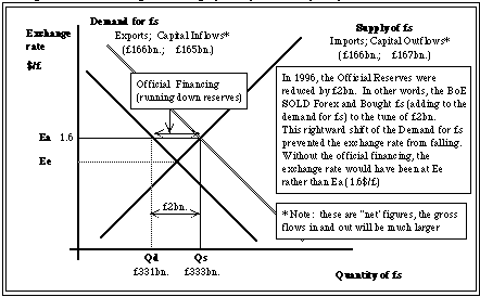 Demand
: Ceteris paribus, exports and capital inflows will be greater
the lower the exchange rate - demand curve slopes downwards.
Demand
: Ceteris paribus, exports and capital inflows will be greater
the lower the exchange rate - demand curve slopes downwards.
Supply : ceteris paribus, will be greater the higher
is the exchange rate - the supply curve slopes upwards.
Equilibrium exchange rate balances exports plus capital inflows
with imports plus capital outflows.
Exchange rate managed by BoE control of Forex reserves, and
also through borrowing (repaying) loans from foreign banks.
Dforex and Sforex are also affected by Incomes (Y) and Interest rates
-
Increasing Income shifts Sf right (increasing demand for imports) -> e.r.
depreciation or BoP deficit
-
Increasing Interest rates shift Sf left (discouraging capital outflows),
and Df right (encouraging capital inflows -> e.r. appreciation or BoP surplus
Monetary Policy more powerful under floating exchange rates than fixed:
Expansionary monetary policy:
-
Increases Y
-
Reduces r
-
depreciates e.r -> more expensive imports, more competitive exports ->
further expansionary effect.
-
more likely to generate inflation
Purchasing Power Parity Theory of exchange
rates - freely floating (unmanaged) exchange rates will adjust in
response to trade-driven demands and supplies of currencies so that (or
until) the prices of the same goods are the same in all countries.
The prices of an identical 'basket' of goods and services
should be the same in all countries - freely floating exchange rates will
adjust to ensure that this is the case - the exchange rates which
would produce this result are known as the 'purchasing power parity' rates
(ppp rates).
This theory relies simply on the pursuit of profitable
trading opportunities - there are at least some people or firms who will
take advantage of the opportunities to buy cheap and sell dear and make
a profit. If they can, they will, and will go on doing so until the prices
(and exchange rates) adjust to remove the profitable opportunities.
This pursuit of trading profit is also known as arbitrage -
from the same root as arbitrate - to arbitrate between prices on
the basis of profit opportunities. It is this arbitrage which ensures,
in this simple 'model' or view of the world, the adjustment of prices and
exchange rates to make prices the same in all countries - it is only then
that arbitrage opportunities are eliminated.
The Economist magazine regularly publishes (at least
once a year) its Big Mac index of exchange rates based on this principle
- what would the exchange rate have to be to make the price of a Big Mac
the same? The answer is a close approximation to the PPP rate between the
two countries.
Back to Contents.
6. MacroEconomic Management:
6.1. The Basics
Economies tend to cycle between booms and recessions:
-
Boom -> rising incomes fueling expectations of further growth.
-
Limited by:
-
capacity constraints -> inflation, depreciation of e.r., increased
uncertainty and pessimism about future prospects plus prospect of active
policy deflation (increasing taxes, increased interest rates)
-
Monetary constraints: -> rising interest rates and appreciating e.r.
-> slower growth
-
Recession -> stable or falling incomes (slower growth), rising inventories
of unsold goods, increasing layoffs and rising unemployment,
-
Limited by:
-
falling prices encouraging consumption and falling wages or availability
of unemployed labour encouraging entrepreneurs to expand,
-
by offsetting macroeconomic policies
-
falling interest rates discouraging saving and encouraging investment
-
increased government spending (social security payments etc.) and lower
taxes encouraging income growth
Counter-cyclical macro-management: (trying to actively predict
and counter-act these cyclical tendencies) Problematic because:
-
information on the current state of the economy is always out
of date, -> response to past conditions, rather than current
conditions;
-
time lags between monetary or fiscal levers and their effects on
the economy substantial and variable. Monetary Policy
an advantage - changed more frequently and easily than Fiscal Policy;
-
the structure of the economy - crudely summarised as the slopes
of the IS and LM curves - is always uncertain;
-
expectations conditon responses - expectations that booms will be
exagerated and be followed by substantial recessions will lead to different
responses from expectations that booms will be slow and longer and less
prone to sudden reversals: so the cyclical behaviour of economies
becomes self-perpetuating.
Active counter-cyclical management tended to exacerbate rather than ameliorate
economic cycles - boom/bust economies. Prefered option now:
-
Automatic [Fiscal] Stabilisers: taxes which increase and goverment
spending items which decrease as incomes grow - and vice versa, so that
booms and busts are self-limiting (e,g, progressive taxation - rising with
incomes, or spending-related taxes, withdrawing more as spending increases
(VAT, excise duties), and also government spending on unemployment benefit
and social security (providing all incomes are rising and not just some)).
-
Responsible Monetary Policy: aimed at purposive adjustment of interest
rates to prevent both inflation and recession - to achieve a low and stable
inflation rate.
Inflationary (boom) situation:
Deflationary (recession) situation:
6.2 Which is more effective?
Fiscal or Monetary Policy?
Experiments with the IS/LM model should clearly show that the effectiveness
of Fiscal and Monetary Policies in governing (managing) the circular flow
of income depend on the slopes of the IS and LM curves.
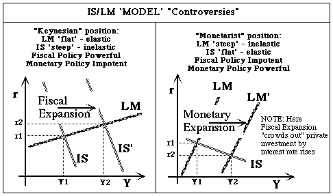
Slopes of the IS and LM Curves:
The IS curve depends on the sensitivity (responsiveness) of aggregate
demand to changes in the rate of interest. It will be flatter the more
responsive aggregate demand (the expenditure loop of the CFoI) is to changes
in the interest rate. On the other hand, if aggregate demand (consumption
plus investment) mostly depend on the current state of the economy and
feelings or expectations about future incomes and spending (growth), then
interest rates may be relatively unimportant in determining aggregate demand,
and the IS curve will be steep.
The LM curve depends on the sensitivity (responsiveness) of money
demand to income - the more responsive the demand for money is to income
changes, the steeper is the LM curve. It is also the case that the more
responsive the demand for money is to interest rates, (the more elastic
the demand for money w.r.t interest rates) the flatter is the LM curve.
Scenario 1 - the classic Depression
-
If investors are "shy" of investing in expanded capacity because they are
unsure about the growth prospects for the economy rather than deterred
by the level of interest rates, the IS curve will tend to be steep (Keynes
referred to the "animal spirits" of business leaders being more important
to investment decisions than the rate of interest).
-
If, at the same time, the economy is stuck in a depressed state with consumers
tending to save more in the face of uncertainty about the future, hence
not increasing the demand for money much as incomes grow, then the LM
curve will tend to be flat.
-
If, in addition, the financial markets are following traditional patterns
of "portfolio management", seeking security and reliability from financial
and physical assets rather than "quick" profit or capital gain, then the
demand for (speculative or idle) balances will be insensitive to interest
rate changes and the LM curve will be flat
This is the story (approximately) for the Great Depression, and much of
the 50s and early 60s - power to Fiscal Policy and Money does not matter
much. If you want to get out of a 1930s type depression, then the Keynesian
solution of demand management works- kick start the depressed economy through
increased government spending over and above taxation receipts.
Scenario 2 - the more modern economy
-
If interest rates are important to investment decisions, then the IS
curve will tend to be flatter.
-
If incomes are expected to grow and personal savings are largely pre-determined
through current income levels (through mortgages, insurance premiums and
pension contributions), then increases in incomes may well be associated
with substantial increases in demand for money - as discretionary incomes
increase. So the LM curve will be steeper since increased demands
for money against a fixed supply will increase the interest rate.
-
As financial markets become more sophisticated and communications make
transactions faster and cheaper, and as the volumes of cash financial institutions
have to deal with increase, so financial portfolio management by large
companies may become more interest sensitive, making the LM curve steeper.
These developments during the seventies may well have made the economy
more sensitive to monetary management and correspondingly less sensitive
to fiscal policy. Power shifts towards Monetary Policy and away
from Fiscal Policy.
Effect of inflation: Notice, if there is inflation in
the economy, then this will reduce the value of money in terms of its purchasing
power, which will mean that more money is required to finance any given
level of transactions or level of real national income. This means that
the supply of money in real terms is reduced, shifting the LM curve to
the left, increasing interest rates and reducing the level of national
income.
Inflation will thus tend to reduce income and increase unemployment
- so long as monetary policy is kept reasonably tight. Overheating (expanding)
the economy will, in these conditions, generate stagflation (both
inflation and increased unemployment) - the typical economic condition
in the UK during the 1970s.
6.3 Inclusion of
Forex Market:
As the economy expands, and national income grows, there is a
tendency for imports to expand faster than exports, and for the Balance
of Trade to move into deficit. This would lead to a depreciation
of the exchange rate. To maintain the exchange rate, the monetary authorities
could (should?) increase interest rates to encourage capital inflows and
discourage capital outflows on the capital account of the Balance of Payments,
thus offsetting the current account deficit.
Thus we may also include an exchange rate equilibrium condition
on the IS/LM diagram, which shows this necessary relationship to
keep exchange rates constant. This is drawn in the following diagram
as the B/C curve - showing an equilibrium exchange rate at some
fixed rate achieved through the balance of the Balance of Trade
and the Capital account of the Balance of Payments.
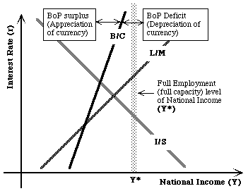
Thus, any point to the left of the BC curve indicates a Balance of Payments
surplus at that level of Y and r, and an appreciating currency under a
floating exchange rate regime. Any point to the right of the BC curve indicates
a balance of payments deficit and a depreciating currency. As the currency
depreciates,
so BC shifts rightwards. As the exchange rate
appreciates,
so BC shifts left.
This diagram also includes the 'target' of full employment or full capacity
National Income (Y*). The implication is that this economy as pictured
is not yet at equilibrium at full employment - nor is there yet a consistent
equilibrium at any level of national income at which all three major markets
(goods, money and forex) will be at equilibrium. It needs managing!
One obvious management tool is to allow the exchange rate to depreciate
- shifting the B/C curve to the right.
The market mechanism (under floating exchange rates) can be expected
to shift the BC curve to the right, as the currency depreciates towards
the money/goods equilibrium (intersection of the IS and LM curves). As
it does so, there may be some inflation triggered by the depreciation,
which would shift the LM curve to the left, raising interest rates. But
this new equilibrium would not be at full employment - it would lie to
the left of Y*. The economy would now have to rely on one of two major
responses:
-
an automatic (market-driven) shift of the IS curve to the right, triggered
by the exchange rate depreciation (making exports more competitive and
imports less competitive with domestic goods) and entrepreneurs in
the economy taking advantage o spare or idle capacity in the economy and
investing in new plant, and also cutting prices to sell unsold stocks (reducing
the price level and allowing the LM curve to shift back to the right.
-
a proactive monetary and fiscal policy combination - shifting either or
both of the IS and LM curves to the right - to hit full employment.
Economies might not adapt and adjust themselves very quickly - so this
economy could stay stuck in an under-employed condition for some time.
So there is a strong temptation for governments to take the proactive line
and expand the economy with either fiscal or monetary policy or both. The
problem is that governments often get this wrong and over-shoot - so generating
inflation as the 'natural' equilibria meet to the right of Y*.
Back to Macro Contents.
Back to AEF811 Index.