Home
Up
Water Resources
Rainfall Modelling
Climate variability
Historical Drought

Published in:

Fowler, H.J., Kilsby, C.G., and O’Connell, P.E. 2000. A stochastic rainfall model for the assessment of regional water resource systems under changed climatic conditions. Hydrol. Earth Sys. Sci., 4, 261-280. [Abstract]

Fowler, H.J., Kilsby, C.G., O’Connell, P.E., and Burton, A. 2005. A weather-type conditioned multi-site stochastic rainfall model for the generation of scenarios of climatic variability and change. Journal of Hydrology, 308(1-4), 50-66. [Abstract]

Burton, A., Kilsby, C.G., Fowler, H.J., Cowpertwait, P.S.P. and O’Connell, P.E. 2008. RainSim: A spatial temporal stochastic rainfall modelling system. Environmental Modelling and Software, 23, 1356-1369.  [Abstract]

This work developed a stochastic rainfall modelling approach based on a linkage to weather type information. A semi-Markov based weather generator was coupled to the Neyman-Scott Rectangular Pulses (NSRP) model developed by Cowpertwait (see references). This method was found to be extremely powerful as it permitted investigation into the impacts of change in weather type persistence or frequency, as well as the rainfall statistics associated with that weather type.

The NSRP Model

The Neyman-Scott Rectangular Pulses (NSRP) model is a clustered point process model. The model parameters broadly relate to underlying physical processes and the model is capable of preserving the statistical properties of a precipitation time series over a range of timescales. For mathematical convenience, some assumptions about the behaviour of raincells have been made. Namely, that rain cells are discs with a random radius and that the location of the disc centres are given by a spatial Poisson process.

 The model considers a catchment of finite area, A, in the x-y plane. Storm origins occur in a Poisson process of rate l, the arrival times being the same at any point on the x-y plane (Figure 1). The arrival of a storm origin at a catchment implies that the physical conditions necessary for precipitation have been met. However, rain only occurs at points covered by rain cells.

Time

Figure 1 The storm origin arrival process

Each storm origin generates a random number (C) of cell origins (Figure 2). The spatial positions of the disc centres are given by a Poisson process of rate r, so that the number of disc centres in a catchment of area A is a Poisson random variable with mean rA. If t is the arrival time of the storm origin and s (>t) is the starting time for a rain cell generated by the origin, then s-t (the waiting time for each cell origin after the storm origin) is taken to be an independent exponential random variable with parameter b, so that the arrival times of cells follows a Neyman-Scott process. No cell origin is located at the storm origin.

Rain cells

Catchment

Figure 2 Graphical representation of the rain disks in the spatial-temporal model

Each cell origin is classified as one of n types, where a_i is the probability that a cell origin is of type i (where i = 1,...,n). The radius R_i of a type i cell is an independent random variable with parameter g_i. A rectangular pulse is associated with each cell origin (Figure 3), depending upon the cell type defined previously. The duration of the pulse is an independent exponential random variable with parameter h, and the intensity of the pulse is an independent random variable X_i for type i cell origins, remaining constant over the lifetime of the cell and the area of the disc.

Time

Figure 3 Graphical representation of precipitation pulses produced at raincells

The total precipitation intensity at a time t and point m is then the sum of the intensities of all the active rain cells at time t that overlap point m (Figure 4). If Y_i^(m)(t) is the total precipitation intensity at time t and point m given by the NSRP(n) model (sometimes called the Generalised NSRP model), and X⁽ⁱ⁾_m,t(u,s) is the precipitation intensity at time t and point m due to a type i cell with centre a distance u from m and starting time t - s, then:

The total intensity at time t and point m, Y^(m)(t), is the sum of the intensities of all cells active at the time t and overlapping m, i.e.

The mean number of cells per storm is denoted as m_c and E(X_i) as m_i. The model is thus a generalised form of the Neyman-Scott Rectangular Pulses model with n cell types.

Time

Figure 4 The calculation of the total precipitation intensity at a time t and point m

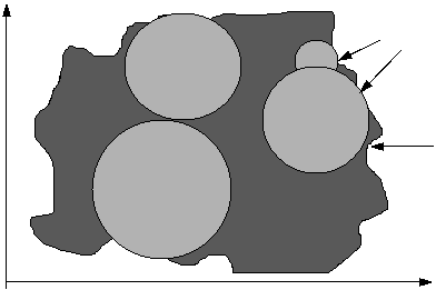
Figure 5 Different cell types represented by the model

As with a single-site model, cells can be classified into different types. Cowpertwait and O’Connell (1997) suggest that the determination of the number of cell types to be included in the model can be guided by observing physical characteristics of the precipitation process. The simplest possible model uses only one cell type but the literature suggests that the precipitation field can be broadly classed into two types; convective and stratiform precipitation (Figure 5). The simplest model would contain only one cell type. However, in a two cell model type 1 cells would be interpreted as ‘heavy’ short-duration convective cells and type 2 cells as ‘light’ long-duration stratiform cells.

Development of a weather type link

The Lamb weather types were grouped using k-means clustering and optimised using a variance minimisation algorithm. This gave 6 weather 'states': winter-anticyclonic (WA), winter-northerly (WN), winter-westerly (WW), summer-anticyclonic (SA), summer-northerly (SN) and summer-westerly (SW). Summer is defined as April to September and winter as October to March. Note that the northerly weather state can also be thought of as 'easterly'.

Here, a semi-Markov process is used to model the occurrence and persistence of weather states. At an initial time, an initial state is entered. After a random duration within that weather state, defined by a distribution fitted to the observed persistence probability distribution, the model enters the next state. This process continues with a randomly defined duration within this state and then a transition to the next state. One-day transition probabilities are defined in a matrix based on observed data. The gamma distribution was found to provide the best fit to the observed persistence probability distribution for each weather state.

Table 1 Observed and simulated total number of days in 114 years of each weather state. Difference refers to the difference between average simulated and observed values (i.e. average – observed). Anomaly yr^-1 refers to the number of days per year of each weather state that are over or under-estimated by the model (i.e. difference/114).

This model was found to produce good simulations of weather state occurrence and persistence when compared to the historic past (Table 1, Figure 6).

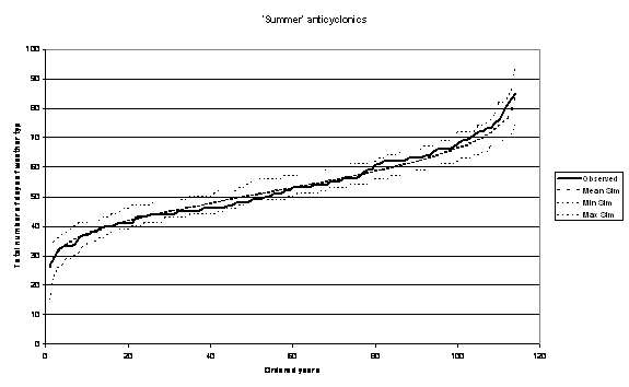
Figure 6 Total number of days occurrence of ‘summer’ anticyclonics for 114 years shown in an ordered sequence with boundary limits.

This was then used to drive the NSRP model - the details on how this is done are shown in the appendix of Burton et al. (2008) and as below:

STNSRP Simulation conditional on weather types

A derivative of the RainSim V2 model was able to generate multisite rainfall with the STNSRP process directly conditioned a daily time series of Lamb weather types (LWTs) (Fowler et al., 2000; 2005). To achieve this, the typical monthly parameterisation was discarded in favour of one using six atmospheric states, each representing both a class of LWTs and a season. This appendix clarifies the NSRP modelling treatment of this conditioning and highlights the modelling issues arising from this approach.

A semi-Markov chain process, conditioned by season, generated a daily time series of atmospheric states (Fowler et al., 2000). Provided a parameter set has been obtained for each state, a particular parameter set is used according to the atmospheric state corresponding to that day. Following the origin of a preceding storm, at say t = 0, it is necessary to estimate when the next storm will occur in the STNSRP process. If the storm arrival rate is constant with parameter, λ₀, then the time of the next storm, t_s, will simply arise from the Poisson process as a random variable with distribution function:

                                                                                 (A)

The parameterization is different in different periods according to the conditioning time series of daily atmospheric states (or in the standard model, calendar month), so the arrival rate may change to λ₁ at time t₁. If the parameterization is on a calendar month basis in a seasonal climate, a storm simulated in a subsequent month by Equation A could be simulated with the new parameters with little introduction of error. However, in a seasonal climate or for daily varying parameterisations as here, more care must be taken with the sampling of the time of storm occurrence. Otherwise dry periods may persist beyond their true extent and daily changes in parameterization will not be correctly modelled as inter-storm periods may be much greater than the daily time scale at which weather states are modelled. Storm arrival is therefore simulated as a piecewise uniform Poisson process.

If t_s is simulated as greater than time t₁ using Equation A1 then there is no storm in the current period and instead the storm arrival sampling is restarted at t₁ with the new value of λ₁. The distribution of this process is given in Equation B for this case. Similarly if the second period finishes at time t₂ with a change to λ₂, Equation C can be used.

                                                                           (B)

                                                                          (C) 

For example in the case of several relatively dry periods followed by a wet one, this sampling should be repeated period by period until the correct storm origin can be located. Note that if λ₁ = λ₀, which can be derived from Equations A and B, simply reduces to Equation A. That is, the storm arrival in two consecutive periods with the same arrival rate using this sampling procedure is the same as in a longer period with that rate, as is required. Once a storm origin is simulated, the remaining properties of the storm are simulated using the parameterisation relating to that period.

A consequence of this modelling methodology is that the final effects of a simulated storm may lag the origin by several days. For example, simulation of a dry period is likely to be biased wet by a preceding wet period. Therefore the identification of observed rainfall statistics and model parameterization for each atmospheric state is difficult and must be carefully carried out (see Fowler et al., 2000; 2005 for further details).

Benefits of this approach

1. Transferable methodology for classification, weather state simulation and precipitation modelling: limited parameter recalibration is needed for application to another region.

2. Physical basis: may be applied successfully to other areas where LWTs are relevant.

3. Allows meaningful re-parameterisation for future climates.

4. Allows production of correlated regional models for large spatial domains.

References

Cowpertwait, P.S.P. 1991. Further developments of the Neyman-Scott clustered point process for modelling rainfall. Water Resour. Res., 27, 1431-1438.

Cowpertwait, P.S.P. 1994 A generalized point process model for rainfall. Proc. R. Soc. Lond. A, 447, 23-37.

Cowpertwait, P.S.P. 1995 A generalized spatial-temporal model of rainfall based on a clustered point process. Proc. R. Soc. Lond. A., 450, 163-175 

Cowpertwait, P.S.P., O’Connell, P.E., Metcalfe, A.V. and Mawdsley, J.A. 1996a. Stochastic point process modelling of rainfall. I. Single-site fitting and validation. J. Hydrol., 175, 17-46.

Cowpertwait, P.S.P., O’Connell, P.E., Metcalfe, A.V. and Mawdsley, J.A. 1996b. Stochastic point process modelling of rainfall. II. Regionalisation and disaggregation. J. Hydrol., 175, 47-65.

Cowpertwait, P.S.P. and O’Connell, P.E. 1997. A Regionalised Neyman-Scott Model of Rainfall with Convective and Stratiform Cells. Hydrol. Earth Sys. Sci., 1, 71-80.